> {-# LANGUAGE MultiParamTypeClasses,FunctionalDependencies,FlexibleInstances,GeneralizedNewtypeDeriving #-}

> module Main where

> import Test.QuickCheck
> import qualified Data.Map as M
> import Control.Monad
> import Ratio

> infixl 5 .+
> infixl 6 .*
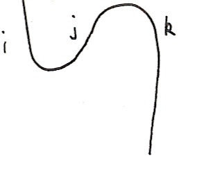
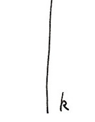
As I've mentioned previously, we need to choose values for our pieces of knot or tangle so that when they're combined together we get something that tells us about the knot or tangle, not the diagram. For example, suppose our diagram contains this piece:

That piece is isotopic to:

We want any kind of evaluation of our diagram to be independent of which one of these we've chosen. In other words, among other things we need this function:
> cupcap i = do
>   (j,k) <- cap
>   cup (i,j)
>   return k
to equal this function:
> straight i = do
>   return i
I've already said how in the vector space monad, these correspond to summations, so really we want these two expressions to be equal (using the summation convention):
MijNjk=δik
(δik is 1 if i=k and zero otherwise, ie. the identity matrix.)
The left hand side is just the rule for multiplying matrices. So we require M to be the inverse of N.
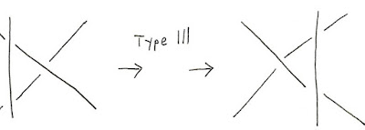
Now we can start on some real knot theory. There is a collection of 'moves' we can perform on a diagram called Reidemeister moves. Here are diagrams illustrating them:


There are three types of move that we call type I, type II and type III.
These diagrams are intended to show changes we can make to a part of a bigger knot or tangle. It's not hard to see that these are isotopies, they're just simple operations we can perform on a knot or tangle by moving the string a little bit. If you perform one of these moves on a knot or tangle then you should end up with merely a different diagram representing the same knot or tangle. Each of these corresponds to an equality of monadic expression, or an equality of summations. But the really important part is that these are all you need to consider. Every isotopy can be constructed out of these moves. So if we can satisfy the corresponding equalities of expressions then we automatically have a knot invariant that tells us about the underlying knot or tangle, not just the diagram.
Unfortunately, there's a catch. Satisfying the equality for a type I move is too onerous. So we'll just concentrate on type II and III. But the good news is that it doesn't matter, there are workarounds.
Let a be an unknown complex number. We're going to build expressions from a but they're all going to be polynomials in a and its reciprocal, like a+a^2-3/a. These are known as Laurent polynomials and I pointed out recently that I can use the Group type class to represent them.
> i = 0 :+ 1
> newtype Z = Z Int deriving (Eq,Ord,Show,Num)
> type Poly = V (Complex Rational) Z
In other words, elements of Poly are weighted linear combinations of integers. We can think of each integer n as representing an and the weights being coefficients of these powers. Amazingly the group multiplication multiplies these things out correctly.
a and ia represent a and a-1.
> a = return (Z 1) :: Poly
> ia = return (Z (-1)) :: Poly
We can now satisfy the type II and III Reidemeister moves with these definitions:
> cup :: (Bool,Bool) -> V Poly ()
> cup (u,v) = case (u,v) of
>   (False,True) -> (-i .* ia) .* return ()
>   (True,False) -> (i .* a) .* return ()
>   otherwise -> zero

> cap :: V Poly (Bool,Bool)
> cap = (-i .* ia) .* return (False,True) .+ (i .* a) .* return (True,False)

> over :: (Bool,Bool) -> V Poly (Bool,Bool)
> over (u,v) = a .* do
>   () <- cup (u,v)
>   cap
>   .+
>   ia .* return (u,v)

> under :: (Bool,Bool) -> V Poly (Bool,Bool)
> under (u,v) = ia .* do
>   () <- cup (u,v)
>   cap
>   .+
>   a .* return (u,v)
(I'm making the V monad do double duty here. I'm using it to represent the Laurent polynomials, but I'm also using it to represent vectors over the Laurent polynomials.)
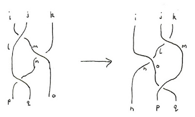
For example, here's what a type III move looks like if we try to arrange things nicely in terms of our standard 'components':

That gives rise to the two functions
> left (i,j,k) = do
>   (l,m) <- under (i,j)
>   (n,o) <- over (m,k)
>   (p,q) <- over (l,n)
>   return (p,q,o)
and
> right (i,j,k) = do
>   (l,m) <- over (j,k)
>   (n,o) <- over (i,l)
>   (p,q) <- under (o,m)
>   return (n,p,q)
whose equality can be tested with
> test1 = quickCheck $ \(x,y,z) -> left (x,y,z)==right (x,y,z)
I'll leave checking the type II rule as an exercise.
With these defintions we can take any knot diagram and compute a value for it. Note that because a not has no loose ends we have no inputs and no outputs so the result won't be a function but a value, a polynomial in a and its reciprocal. This is known as the Bracket Polynomial.
As mentioned above, the bracket polynomial fails to be a knot invariant. Two diagrams related by type I moves will have different bracket polynomials. With a little bit of sleight of hand we can apply a fudge factor to l with those extra loops and we end up with the Jones polynomial. As that's not my main goal here, I'll let you read how to use the writhe get from the bracket polynomial to the Jones polynomial at Wikipedia. But do I want to make another digression.
It's tricky to define knot invariants. The problems is that knots are topologically invariant in the sense that you can deform a knot in lots of ways and it's still the same knot. This rules out most attempts at using the geometry of a knot to define an invariant. Just about any geometrical feature you find in a particular configuration will be ruined by deforming the knot. But here's an idea: suppose you could compute some geometrical property from a particular curve representing a knot and then find the average of that value for all possible curves representing the same knot. Then we'd get a knot invariant as it wouldn't depend on a particular choice of representative curve. But there's a catch. We need to average over an infinite space, the space of all curves representing a knot. On the other hand, there is a perfectly good tool for averaging over infinite sets: integration. But there's another catch: the space of all curves representing a knot is very large, infinite dimensional in fact, and we don't have very good theory for how to do this. At least mathematicians don't. But physicists integrate over spaces of paths all the time, ever since Feynman came up with the path integral. Amazingly, Ed Witten showed that tere was already a physical model that fit the bill: Chern-Simons theory. In fact, Witten showed that the Jones polynomial, which as I've already mentioned came originally out of statistical mechanics, could be derived from this theory.
Anyway, enough of that digression. In the next installment I'll show how the above can be modified for use with tangles and give my final algorithm.
In the last installment (I think) I'll show how we can derive the rational number for a tangle using the bracket polynomial.
The following is the 'library' behind the code above. Most of it is simply built up from what I've said in recent weeks.
> swap (x,y) = (y,x)

> class Num k => VectorSpace k v | v -> k where
>     zero :: v
>     (.+) :: v -> v -> v
>     (.*) :: k -> v -> v
>     (.-) :: v -> v -> v
>     v1 .- v2 = v1 .+ ((-1).*v2)

> data V k a = V { unV :: [(k,a)] } deriving (Show)

> reduce x = filter ((/=0) . fst) $ fmap swap $ M.toList $ M.fromListWith (+) $ fmap swap $ x

> instance (Ord a,Num k) => Eq (V k a) where
>   V x==V y = reduce x==reduce y

> instance (Ord a,Num k,Ord k) => Ord (V k a) where
>   compare (V x) (V y) = compare (reduce x) (reduce y)

> instance Num k => Functor (V k) where
>     fmap f (V as) = V $ map (\(k,a) -> (k,f a)) as

> instance Num k => Monad (V k) where
>     return a = V [(1,a)]
>     x >>= f = join (fmap f x)
>         where join x = V $ concat $ fmap (uncurry scale) $ unV $ fmap unV x
>               scale k1 as = map (\(k2,a) -> (k1*k2,a)) as

> instance Num r => MonadPlus (V r) where
>     mzero = V []
>     mplus (V x) (V y) = V (x++y)

> instance (Num k,Ord a) => VectorSpace k (V k a) where
>     zero = V []
>     V x .+ V y = V (x ++ y)
>     (.*) k = (>>= (\a -> V [(k,a)]))

> e = return :: Num k => a -> V k a
> coefficient b (V bs) = maybe 0 id (lookup b (map swap (reduce bs)))

> diag a = (a,a)
> both f g (a,b) = (f a,g b)

> class Group m a where
>     unit :: () -> m a
>     counit :: a -> m ()
>     mult :: (a,a) -> m a
>     comult :: a -> m (a,a)
>     anti :: a -> m a

> instance Monad m => Group m Z where
>     unit _ = return (Z 0)
>     counit _ = return ()
>     mult = return . uncurry (+)
>     comult = return . diag
>     anti = return . negate

> newtype Identity a = I a deriving (Eq,Ord,Show)

> instance Monad Identity where
>     return x = I x
>     I x >>= f = f x

> data K = K Rational Rational deriving (Eq,Show)

> instance Num K where
>   K a b + K a' b' = K (a+a') (b+b')
>   K a b * K a' b' = K (a*a'+2*b*b') (a*b'+a'*b)
>   negate (K a b) = K (negate a) (negate b)
>   abs _ = error ""
>   signum _ = error ""
>   fromInteger i = K (fromInteger i) 0

> instance Num k => Num (V k Z) where
>   a + b = a .+ b
>   a * b = do
>       u <- a
>       v <- b
>       mult (u,v)
>   negate a = (-1) .* a
>   fromInteger n = fromInteger n .* return 0
>   abs a = error ""
>   signum a = error ""

> data Complex a = (:+) { realPart :: a, imagPart :: a } deriving (Eq,Show)

> instance Num a => Num (Complex a) where
>   (a :+ b) + (a' :+ b') = (a+a') :+ (b+b')
>   (a :+ b) * (a' :+ b') = (a*a'-b*b') :+ (a*b'+a'*b)
>   negate (a :+ b) = (-a) :+ (-b)
>   fromInteger n = fromInteger n :+ 0
>   abs (a :+ b) = undefined
>   signum (a :+ b) = undefined

> instance Fractional a => Fractional (Complex a) where
>   recip (a :+ b) = let r = recip (a*a+b*b) in ((a*r) :+ (-b*r))
>   fromRational q = fromRational q :+ 0

> instance Ord (Complex Float) where
>   compare (a :+ b) (c :+ d) = compare (a,b) (c,d)
2 comments:
Beautiful. i find it intriguing that the π-calculus model has no trouble with R1 and R2, but has to introduce non-trivial machinery to get R3, while your model gets R2 and R3, but finds R1 more problematic.
If you circumscribe a ball around the locus of activity in an R-i move, you see that the laws are about crossings that make no difference to an observer on the outside of that ball. Specifically, if you think of the observer as capable of seeing signal pulses on a wire that is twisted into a knot, the Reidemeister moves will preserve signal patterns on the wires. For example, an observer who has concluded a wire acts as a perfect infinite capacity buffer, will conclude that a loop acts like a wire -- this is the observational content of R1.
R1 and R2 treat the introduction/elimination of crossings that do not change the experience of the observer while R3 is about a commutativity property. This commutativity property is very tricky for bisimulation to capture.
leithaus,
The failure of the type I moves can be viewed in terms of framed knots. It arises naturally when looking at the Chern-Simons model, so there's a deep significance to this 'failure'.
Post a Comment