Untangling with Continued Fractions: Part 3

It's time to return to the vector space monad. But first, after some Haskell preamble, I need to talk about the Einstein summation convention.

> {-# LANGUAGE MultiParamTypeClasses,FlexibleInstances,FunctionalDependencies #-}

> module Main where

> import qualified Data.Map as M
> import Control.Monad
> import Test.QuickCheck

> infixl 4 .+
> infixl 4 .-
> infixl 5 .*

We're going to be dealing with multidimensional arrays of values that I'll call tensors. We can refer to the individual elements of these arrays by providing tuples of indices drawn from some set of indices. For example we might refer to the elements of a 10 by 10 array by using pairs of indices, each drawn from the set {0,1,2,...,9}. We'll write some indices as subscripts and some as superscripts. Here are some examples: vⁱ, w_j,T^ij,W^ij_kl. vⁱ means the ith value in array v, T^ij means the (i,j)-th element of T and so on.

We can form sums over such indices like this

Σ_jkT^ijW_jkv^k

where the sum is over the corresponding index sets for j and k.
The Einstein summation convention is simply this: if an expression has an index repeated once as a subscript and once as a superscript then we implicitly assume a sum over the index without writing the summation symbol. So the above expression becomes simply

T^ijW_jkv^k

The vector space monad allows us to express something similar using do-notation. Let's use the type Bool for our index set, so we're selecting elements of our arrays using the values {False,True} rather than integers. Let e_i be the (2-dimensional) vector with the property that its j-component is 1 for j=i and 0 for j≠i. In do-notation this is represented by return i. We use superscripts to indicate the components of a vector so the components of e_i are e^j_i. We can write the vector v=3e_False-5e_Truea, with components (3,-5) as

> v :: V Float Bool
> v = 3 .*return False .- 5 .*return True

Dual to vectors we have covectors. You can think of these as linear functions that consume vectors and return reals. We can define a basis of covectors fⁱ with the property that fⁱ(e_j) is 1 for i=j and 0 otherwise. In our Haskell code it'll be more convenient to think of covectors as mapping vectors to the one-dimensional vector space whose basis element is labelled by (). When we make a vector using an expression like return True, that True is a constructor for the type Bool. We expect to use the dual operation for covectors, and that dual is case analysis. So, for example, we can write w = f^False+2*f^True, wih components (1,2), as

> w :: Bool -> V Float ()
> w i = case i of
>   False -> return ()
>   True -> 2 .* return ()

Applying w to v gives the expression vⁱw_i using the summation convention. Using do-notation it looks like

> vw :: V Float ()
> vw = reduce $ do
>   i <- v
>   w i

The point to note is that just like with the summation convention, we don't need to explicitly sum over i. i serves as a kind of iterator object and a vector v automatically supplies i with values in the appropriate range. w then consumes i. So we can translate the summation convention to do-notation by thinking of upper indices corresponding to places that iterators can emerge from, and thinking of lower indices as places where iterators can be consumed.

Another example is matrix representing a transformation of a vector to a vector. It must consume one iterator and emit another one. In the Einstein summation convention such a transformation might be written rⁱ=Mⁱ_jv^j. We could write a simple 2D 2x scale and 90 degree rotation matrix as

> m :: Bool -> V Float Bool
> m j = case j of
>   False -> 2 .*return True
>   True -> -2 .*return False

We can then write the transformation as

> r = do
>   j <- v
>   i <- m j
>   return i

Another simple example is an inner product. We can represent the ordinary dot product as a matrix d_ij and write the square length of v as v . v = d_ijvⁱv^j. We can implement this as

> v2 = do
>   i <- v
>   j <- v
>   d (i,j)

where we define

> d (i,j) = case (i,j) of
>   (False,False) -> return ()
>   (True,True) -> return ()
>   otherwise -> mzero

Similarly, tuples of superscripts correspond to iterators that are tuples of indices.

With that in place, we're now in a position to consider what monadic notation for knots means in the vector-space-over Bool monad. Essentially what we're doing is representing 'components' of a tangle or knot, the cups, caps and crossings, as tensors. When we glue these components with labels we're forming sums. In fact, each labelled edge connecting two components corresponds to an index and so we can think of it as possibly taking two different values, False or True. So the monadic expression corresponds to a sum over all possible ways to assign values from Bool to the indices with a corresponding weight for each term. This should be familiar to some people, it's just like what takes place in statistical thermodynamics. We consider a bunch of particles and form a sum over all of the possible states that those particles could have, with a corresponding weight for each configuration of states. A good example is the Ising model in which electrons sit at the vertices of a regular lattice. Two neighbouring electrons in a ferromagnet tend to want to align the same way, so confgurations in which neighbouring electrons have the same spin will get assigned a higher weight.

In our tangle problem, the trick is to find a magic set of weights with the property that two different summations representing isotopic knots or tangles give the same result. This turns out to be too hard, but we relax it a bit we will be led to one of the most fruitful new approaches in knot theory in recent years - the Jones Polynomial. Vaughan Jones was investigating certain types of model from statistical mechanics and came to realise that some of the equations that were arising were the same ones needed to get suitable weights for knot theory. From this realisation emerged his eponymous polynomial. But, that's all I'll be saying about this polynomial in this post.

Anyway, to make things clearer here's an example:



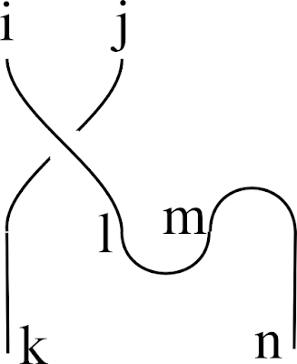
We interpret cap, cup, over and under as the tensors M^ij, N_ij, S^ij_kl and T^ij_kl. In monadic notation we get

> example (i,j) = do
>   (k,l) <- over (i,j)
>   (m,n) <- cap
>   cup (l,m)
>   return (k,n)

With the summation convention in mind this evaluates to:

S^ij_klN^lmM_m,n

and without it we see that all we're doing is computing

Σ_l,mS^ij_klN^lmM_m,n

We can try an elementary choice for our tensors above. We can define M and N to be given by identity matrices:

> cap :: V Float (Bool,Bool)
> cap = return (False,False) .+ return (True,True)

> cup :: (Bool,Bool) -> V Float ()
> cup (i,j) = case (i,j) of
>   (False,False) -> return ()
>   (True,True) -> return ()
>   otherwise -> mzero

We can then choose S and T to simply swap their arguments:

> over,under :: (Bool,Bool) -> V Float (Bool,Bool)
> over (i,j) = return (j,i)
> under (i,j) = return (j,i)

With these choices, the weighting is such that a non-zero weight is assigned to a knot or tangle if and only if all of the labels along a single strand are assigned the same value, in other words we're now summing over ways of assigning labels to entire strands. For rational tangles we can only end up with three possible values corresponding to the three ways the two outputs can be connected to the two inputs. (Straight through, the tangle I called ∞; straight through with a swap, the tangle called -1; and connecting together both the inputs, and both the outputs, the tangle called 0.)

> tangleInfinity,tangleMinus1,tangleZero :: (Bool,Bool) -> V Float (Bool,Bool)
> tangleInfinity (i,j) = return (i,j)
> tangleMinus1 (i,j) = return (j,i)
> tangleZero (i,j) = do
>   cup (i,j)
>   cap

> test1 = quickCheck $ \x -> (example x == tangleInfinity x)
> test2 = quickCheck $ \x -> (example x == tangleMinus1 x)
> test3 = quickCheck $ \x -> (example x == tangleZero x)

Only test2 succeeds so we know example is a tangle that forms its outputs by swapping the inputs.

So even with this simple assignment we're able to extract some basic connectivity information from our monadic representation. With smarter choices we'll get more information, but that's enough for now. We now have the prerequisites and in the next installment we can start doing some proper knot theory.

---

> data V r b = V [(r,b)] deriving (Eq,Show)
> unV (V bs) = bs

> instance Num r => Functor (V r) where
>    fmap f (V bs) = V $ map (\(r,b) -> (r,f b)) bs

> scale x (bs) = map (\(r,b) -> (x*r,b)) bs

> instance Num r => Monad (V r) where
>    return b = V [(1,b)]
>    x >>= f = join (fmap f x)
>        where join x = g $ fmap unV x
>              g (V bs) = V $ concat $ map (uncurry scale) bs

> instance Num r => MonadPlus (V r) where
>    mzero = V []
>    mplus (V x) (V y) = V (x++y)

> class Num r => VectorSpace r v | v -> r where
>    zero :: v
>    (.+) :: v -> v -> v
>    (.*) :: r -> v -> v
>    (.-) :: v -> v -> v
>    v1 .- v2 = v1 .+ ((-1).*v2)

> swap (x,y) = (y,x)
> reduce x = V $ filter ((/=0) . fst) $ fmap swap $ M.toList $ M.fromListWith (+) $ fmap swap $ unV $ x

> instance (Num r,Ord b) => VectorSpace r (V r b) where
>    zero = V []
>    V v1 .+ V v2 = reduce (V (v1 ++ v2))
>    r .* V v = reduce (V $ scale r v)

Untangling with Continued Fractions: Part 2

Recall that I defined a rational tangle to be what you get by starting with a pair of untangled strings whose ends are at infinity and then sliding the strings around as much as you like keeping the ends at infinity. If you don't like the infinity bit, just think of strings inside a sphere with the ends constrained to lie on (but free to slide around) the surface of the sphere. We also insist that the ends end up at the four diagonal directions.

Two rational tangles are considered to be isotopic if you can slide the strings about to turn one into the other, this time keeping the ends of the strings fixed. (Such a motion is called an isotopy.)

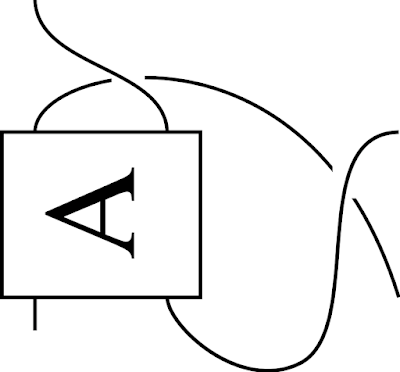
As I've previously mentioned, you only need twists, antitwists and rotations to untangle a rational tangle. Here are the twist operations again:



I'm using a box to represent some unknown tangle. The antitwist really is an inverse for the twist because one followed by the other gives you what you started with once you pull the strings straight:


We can also draw a rotation like this:

Let's call the twist T (so the antitwist is T^-1) and the rotation S and write products of operations from right to left in the usual way. As both S and T are invertible, they generate a group. It's pretty clear that S⁴=1, where 1 is the identity operation. So we don't need a clockwise rotation, we can just use S³.

But here's a surprising fact: S²=1. If we perform a 180 degree rotation on a rational tangle the result might look different at first, but it is isotopic to what we started with. I'll leave you to convince yourself of this, but you can prove it by induction on the number of twists or antitwists you have in your diagram. Try it for simple rational tangles first, maybe real ones made with real string.

Here's an even more surprising fact, (TS)³=1. I can demonstrate this pictorially. Start with he result of applying T:



The result of ST:



The result of TST:



The result of STST:



After TSTST:


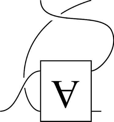
But by sliding one string behind the tangle, allowed in an isotopy, we find that that is isotopic to this:


It's not hard to see that another S brings us back to where we started. (To do that we need to rotate the block labelled A, but that is allowed in an isotopy as we're not moving the ends of the strings.) This means we can write an antitwist in terms of twists and rotations. But it's convenient to keep using antitwists.

So we have S²=1 and (ST)³=1. It can also be proved that any other relationships between S and T can be derived from these using the operations in a group. But this is a well studied group. We can approach it like this. Define two functions s and t by

s(x) = -1/x

t(x) = x+1.

It's easy to show that s²=identity=(st)³. In fact, we have an isomorphism between the group of operations we can perform on rational tangles and the functions we can build with s and t. It goes further.

Take the rational numbers and throw in ∞ to give us the extended rationals. Let s and t act in the usual way on most of the rationals but throw in the extra rules s(∞)=0, s(0)=∞ and t(∞)=∞ to handle infinity. We have defined an action of s and t on the extended rationals. We can exactly parallel this with the rational tangles. Call this tangle 0:



We can reach every rational tangle by applying the operations S and T to 0. But if we replace S with s and T with t then the sequence of s's and t's will give us an extended rational number that labels the tangle. Because S and T obey the same equations as s and t, isotopic knots will end up getting the same extended rational. So we can use extended rationals to label the rational tangles. Here are some examples:

Firstly just an antiwist, T^-1. That corresponds to t^-1(0)=-1.



Two antitwists gives -2:



Composing a 90 degree rotation gives



And applying another antitwist subtracts one again giving:


The name rational tangle is justified.

So, given any any rational tangle we simply need to find the corresponding extended rational and then figure out how to write it as a composition of s's and t's applied to 0. This is more or less the usual technique for finding the continued fraction representation of a rational. And once we know the sequence, we can then apply it in reverse to untangle the tangle.

But there's one catch, how can we go from the monadic representation of a tangle that I described previously to the corresponding extended rational? We'll start on that problem in my next post, but amazingly the vector space monad can be used to do almost all of the work. It's surprising: it's only a short bit of code that works out the untangling operations, but the explication is getting rather long now...

An amazing application of this work is in the study of the untangling of DNA. DNA is a double helix and the two parts of the helix must be separated in order to transcribe it. As you might imagine, the DNA can become incredibly tangled by this process. To deal with this, the topoisomerases snip, manipulate and repair the DNA so as to eliminate these tangles. It was realised that it was possible to work out exactly what operations the topoisomerases were performing by analysing the before and after DNA strings in terms of rational tangles.

The perosn who first figured out this relationship between tangles and rational numbers was the ubiquitous JH Conway.

References

For the proofs missing above, these references should fill in the details:
Rational Tangles, Kauffman and Goldman
Knots and Physics, Kauffman
And if I've lost you above, the following is a nice easy introduction:
Conway's Rational Tangles, Davis
Modeling protein-DNA complexes with tangles

One last thing. I've noticed some, but not all, papers define the twist oppositely from me.

Untangling with Continued Fractions: Part 1

Continuing from before It's time now do discuss the problem of forming a representation of a knot or tangle in machine readable form.

I've defined rational tangles but I should set that in a wider context. A knot is essentially a single closed loop embedded in 3D space and a link is a non-intersecting union of a bunch of these. Any tangle, knot or link can be projected down to 2D space so that you get a finite collection of 'over' or 'under' crossings connected by arcs. You might have to jiggle things around a bit to ensure that you don't get any degeneracies like two separate parts of a knot being projected to the same segment of curve in 2D, but this is always possible. Here's an example of such a 2D projection, a knot diagram, for the photograph I posted last week:

Roughly speaking, two knots or links or tangles are equivalent if you can slide the strings about to get from one to the other without passing one string through another. In the case of rational tangles we have the extra constraint that the free ends mustn't move and must always remain 'at infinity' so you can't pass loops over the end. Given two diagrams for rational tangles, the task is to tell when they represent something equivalent. I'll start on this in a future posting, but for now I just want to consider the problem of getting diagrams like that above into machine readable from. (Incidentally, the rigorous mathematical definition of knot equivalence, ambient isotopy, relies on the notion of finding a continuous bijection between the space around the two knots, not the knot itself.)

We don't need anything particularly clever to form our representation as there is a fairly commonplace way to represent connectons between components using monads. If we have some kind of block with inputs a and b and outputs c and d we can represent this as a line of do-notation looking like

(c,d) <- block (a,b)

Examples of such notation are in Matthew Naylor's article on Lava. We could also use arrows but in this case there is no need.

So now we need to break up a diagram of a rational tangle into components and hook them up, working down the diagram from top to bottom. There are four essential components that can be discerned and I'm calling them cups, caps, overs and unders. Here are the corresponding diagrams for each one:

Cups have two inputs but no output and caps have two outputs and no inputs.

Now all we have to do is label the inputs and outputs of each arc, write the corresponding lines as above, and collect them together in a do-block. Here I've redrawn the above diagram marking the cups and caps with red circles and the overs and unders with green circles.

I've also labelled the inputs and outputs. We can now write the following block of code.

> example (a,b) = do
>   (c,d) <- over (a,b)
>   (e,f) <- cap
>   (g,h) <- over (c,e)
>   (i,j) <- over (f,d)
>   (m,n) <- cap
>   (k,l) <- cap
>   (q,r) <- over (h,k)
>   (s,y) <- over (l,i)
>   (o,p) <- over (n,g)
>   (t,u) <- under (p,q)
>   (v,w) <- under (r,s)
>   (x,z) <- over (y,j)
>   cup (o,t)
>   cup (u,v)
>   cup (w,x)
>   return (m,z)

Note how this block has a pair of inputs (a,b) and a pair of outputs (m,z) corresponding to the strings at the top and bottom. Clearly knots and links should have no inputs or outputs but rational tangles should have a pair of inputs and a pair of outputs. The precise order shouldn't matter as long as you don't try to use a name that isn't yet in scope.

So what monad should we use? It's easy to imagine some kind of state monad that allows us to generate fresh labels for each of the connections and collects up a graph-like representation of our tangle. But the surprise is this: it turns out we don't need to do anything complicated like this. With suitable definitions of cup, cap, over and under, not only does the vector space monad give us the representation we want, it also does most of our computation for us. But first I need to explain the underlying mathematics in an upcoming installment.

Untangling with Continued Fractions: Part 0

A rational tangle is what you get when you take two initially separate lengths of rope and then allow them to interact while keeping the ends 'at infinity'. You're allowed to do whatever tangling you like with the proviso that you can't pass the ends of the ropes through your tangle. We'll also insist that tangles are arranged so that the four loose ends go off in directions corresponding (at least roughly) to the four diagonals. This is, of course, mathematics, so there'll be some idealisation going on too.

Here is an example of a tangle:




My goal over the next few posts is to sketch how these tangles can be classified mathematically and develop a short Haskell program to tell you how to untangle them. Along the way we'll meet a monad that gives a simple embedded language to describe knots and tangles as well as an amazing connection with continued fractions noticed by John Conway. We'll also briefly touch on some statistical thermodynamics, quantum field theory, quantum computing, genetics as well as a little bit of knot theory. Amazingly these subjects are all tied together in surprising ways.

The important idea is that all such tangles can be untangled by composing a sequence of just three operations: a rotation, a twist and an antitwist. A rotation is simply a 90 degree rotation anticlockwise. A twist brings the lower right string over the upper right string so that the upper and lower right strings end up swapping places. An antitwist is the inverse to the twist so that a twist followed by an untwist cancels out. It's a bit like solving Rubik's cube.



If I enter machine readable notation describing the above photo into my program the output should be:

rotate
antitwist
rotate
twist
rotate
antitwist
rotate
twist
rotate
antitwist
antitwist
antitwist

Here is a movie showing how that solution gets played out. That's one initial frame plus 12 more for each of the moves listed above:



(Note that I used bungee cords which are quite rigid so doing a twist would sometimes flip the innards of the tangle itself, for example on the first antitwist. That's allowed. The restriction is that I can't bring the ends into 'the picture' at any point.)

Anyway, it took a while to put that video together so that's all for now. In the next post I'll discuss how we form a machine readable description of the tangle above using monadic do-notation. (It'd be cool if I had some smart image processing code to do this, but alas, we're going to have to enter it by hand.)

Hopf Algebra = Group + Monad

I have two goals in this post. Firstly I want to revisit the vector space monad I've used before. This time I want to show how it provides a great domain specific language for working with multilinear functions on vector spaces. Secondly I want to apply this monad to talk about Hopf algebras. In particular I want to address the issue of why Hopf algebras and groups are actually the same thing. In fact, I want to push this idea to the point where I can use exactly the same code to perform operations in both groups and Hopf algebras. By parameterising the definition of groups in the right way, Hopf algebras appear as if by magic simply by tweaking one parameter. What this means is that if you understand groups and vector spaces, and are comfortable with monads in Haskell, then despite their notoriety as something whose definition is a little opaque, you'll have some idea of what a Hopf algebra is well before the end this post.

Of course there's the question of why anyone would want to know about Hopf algebras. They appear in combinatorics, topology and knot theory, and theoretical physics among other subjects. In fact, there's a review paper on their ubiquity. As topics in mathematics go, this is a hot one.

First some administrivia, because this is, as always, a literate Haskell post.

> {-# LANGUAGE MultiParamTypeClasses,FlexibleInstances,FunctionalDependencies,GeneralizedNewtypeDeriving #-}

> module Main where

> import qualified Data.Map as M
> import Control.Monad
> import Test.QuickCheck

> infixl 5 .+
> infixl 6 .*

> swap (x,y) = (y,x)

Vector Spaces

We'll start with a type class for vector spaces v over a base field k:

> class Num k => VectorSpace k v | v -> k where
>     zero :: v
>     (.+) :: v -> v -> v
>     (.*) :: k -> v -> v
>     (.-) :: v -> v -> v
>     v1 .- v2 = v1 .+ ((-1).*v2)

.+ is vector space addition and .* is scalar multiplication by elements of the base field.

And now I need a concrete instance. I'll be working with vector spaces equipped with a basis. I'll use the obvious representation: a list of pairs of coefficients and basis elements. So 2x-3y is represented as V [(2,x),(3,y)]. Sometimes it will be clearer if I write 2e_x-3e_y. x and y aren't really the basis elements but labels. The e_x and e_y are the actual basis elements. But it's often more readable to write x and y.

> data V k a = V { unV :: [(k,a)] } deriving (Show)

The problem with this representation is that basis elements might appear in any order, the same basis element might appear multiple times, and some basis elements might appear with redundant zero coefficients. We need a suitable definition of equality. (I'm sidestepping the usual issues with Eq and Monad.)

> reduce x = filter ((/=0) . fst) $ fmap swap $ M.toList $ M.fromListWith (+) $ fmap swap $ x

> instance (Ord a,Num k) => Eq (V k a) where
>   V x==V y = reduce x==reduce y

> instance (Ord a,Num k,Ord k) => Ord (V k a) where
>   compare (V x) (V y) = compare (reduce x) (reduce y)

V is a functor. fmap f just applies f to the basis elements.

> instance Num k => Functor (V k) where
>     fmap f (V as) = V $ map (\(k,a) -> (k,f a)) as

Given any type a, V k a is the type of vectors over k generated by elements of a. So V k (V k a) is the type of vectors whose basis elements are themselves labeled by vectors in V k a. We can think of an element of V k (V k a) looking something like 2(2x+3y)-5(3x-y). It's tempting to say this is equal to what we get when we multiply out, but where I wrote '2x+3y' I really meant e_2x+3y. Nonetheless, we can define a function that does the multiplying out. I'll call this function join. So we get a function join :: V k (V k a) -> V k a. In fact, we get a monad.

> instance Num k => Monad (V k) where
>     return a = V [(1,a)]
>     x >>= f = join (fmap f x)
>         where join x = V $ concat $ fmap (uncurry scale) $ unV $ fmap unV x
>               scale k1 as = map (\(k2,a) -> (k1*k2,a)) as

What's really going on here is that the "vector space over basis" functor is a monad in the category Set, but in the category of Haskell types and functions we're stuck with lists.

V k is not just a monad, it's also a MonadPlus.

> instance Num r => MonadPlus (V r) where
>     mzero = V []
>     mplus (V x) (V y) = V (x++y)

So what's the use of making our vector space into a monad? If m is a monad, then any function f:a→mb can be lifted to a function f':ma→mb. f maps the basis elements in a to elements of mb. It's a standard fact about vector spaces that a linear function is completely defined by its value on a basis. f' is the corresponding linear function. So we only need to implement linear functions for basis elements and the function can be automatically lifted to a linear function on the whole vector space. An arrow of the form a→mb is a Kleisli arrow and what I've just argued is that the Kleisli category of the V k monad is the category of vector spaces with basis.

This gives us lots of advantages. For example, we can't accidentally implement a function that isn't linear this way. If we implement the action on a basis, the lift can't help but be linear. Also, working with basis elements rather than the vector space gives us greater flexibility. For example, it'll be easy to form tensor products of vector spaces by directly working with their bases.

Here's the instantiation of the vector space type:

> instance (Num k,Ord a) => VectorSpace k (V k a) where
>     zero = V []
>     V x .+ V y = V (x ++ y)
>     (.*) k = (>>= (\a -> V [(k,a)]))

> e = return :: Num k => a -> V k a
> coefficient b (V bs) = maybe 0 id (lookup b (map swap (reduce bs)))

I could have implemented .* using scale but this definition is more in the spirit of what's to come.

Groups

Now we switch to groups. Here's a first attempt at writing a group type class

> class Group1 a where
>    unit1 :: a
>    mult1 :: a -> a -> a
>    inverse1 :: a -> a

> newtype Z = Z Int deriving (Eq,Ord,Show,Arbitrary,Num)

> instance Group1 Z where
>    unit1 = Z 0
>    mult1 = (+)
>    inverse1 = negate

Now we can try testing some of the group laws. For example

> test_inverse1 a = mult1 a (inverse1 a)
> ex1 = quickCheck (\a -> test_inverse1 a==(unit1::Z))

If we run ex1 we gain some confidence that we have a group. If we want to be more categorial then we need to express as much as possible as compositions of functions. So let's break down test_inverse1 as a composition of elementary operations.

> diag a = (a,a)
> both f g (a,b) = (f a,g b)
> test_inverse2 = uncurry mult1 . (id `both` inverse1) . diag
> ex2 = quickCheck (\a -> test_inverse2 a==(unit1::Z))

There's a nice symmetry in test_inverse2. If we make diag part of the definition of a group that we can make this highly symmetric definition of a group:

> class Group2 a where
>     unit2 :: () -> a
>     counit2 :: a -> ()
>     mult2 :: (a,a) -> a
>     comult2 :: a -> (a,a)
>     anti2 :: a -> a

I've even made a (useless looking) symmetric partner for unit1 and I've renamed the inverse operation as anti, short for antipode. Let's make Z an instance of this class.

> instance Group2 Z where
>   unit2 () = Z 0
>   counit2 _ = ()
>   mult2 = uncurry (+)
>   comult2 a = diag a
>   anti2 = negate

I hope I haven't done anything too tricky yet. This is just the familiar definition of a group except I've made a trivial 'counit' and the diagonal function part of the definition. Now comes the most important step in this post: I'll tweak this definition so that all of the associated functions are now Kleisli arrows:

> class Group m a where
>     unit :: () -> m a
>     counit :: a -> m ()
>     mult :: (a,a) -> m a
>     comult :: a -> m (a,a)
>     anti :: a -> m a

We can now straightforwardly reimplement Z as an instance of this class.

> instance Monad m => Group m Z where
>     unit _ = return (Z 0)
>     counit _ = return ()
>     mult = return . uncurry (+)
>     comult = return . diag
>     anti = return . negate

Apart from writing it monad-agnostically, it's just like before. We can exactly recover what we had before with the help of the identitiy monad.

> newtype Identity a = I a deriving (Eq,Ord,Show)

> instance Monad Identity where
>     return x = I x
>     I x >>= f = f x

Now we can rewrite the group laws. Before checking to see if aa^-1=1 we'll make sure aa^-1=a^-1a.

> test_antipode1 a = do
>     (u,t) <- comult a
>     u' <- anti u
>     mult (u',t)

> test_antipode2 a = do
>     (u,t) <- comult a
>     t' <- anti t
>     mult (u,t')

> ex3 = quickCheck (\a -> lhs a==rhs a) where
>   lhs = test_antipode1 :: Z -> Identity Z
>   rhs = test_antipode2 :: Z -> Identity Z

For aa^-1 we need to compare with the identity. We make an identity by applying unit to (). We could just provide a () but we get something more symmetrical if we construct it using the counit.

> test_antipode3 a = do
>   x <- counit a
>   unit x

> ex4 = quickCheck (\a -> lhs a==rhs a) where
>   lhs = test_antipode1 :: Z -> Identity Z
>   rhs = test_antipode3 :: Z -> Identity Z

We can test associativity easily

> test_assoc1 (a,b,c) = do
>     ab <- mult (a,b)
>     mult (ab,c)

> test_assoc2 (a,b,c) = do
>     bc <- mult (b,c)
>     mult (a,bc)

> ex5 = quickCheck (\a -> lhs a==rhs a) where
>   lhs = test_assoc1 :: (Z,Z,Z) -> Identity Z
>   rhs = test_assoc2 :: (Z,Z,Z) -> Identity Z

In the interest of symmetry, there ought to be a coassociativity law for comultiplication. Here it is:

> test_coassoc1 x = do
>     (u,v) <- comult x
>     (s,t) <- comult v
>     return (u,s,t)

> test_coassoc2 x = do
>     (u,v) <- comult x
>     (s,t) <- comult u
>     return (s,t,v)

> ex6 = quickCheck (\a -> lhs a==rhs a) where
>   lhs = test_coassoc1 :: Z -> Identity (Z,Z,Z)
>   rhs = test_coassoc2 :: Z -> Identity (Z,Z,Z)

One issue is that we've introduced comult without making much demand on it. Here's a law that is obviously true in any group that helps to pin down comult. It's simply evaluating (p,q) →(pq,pq) in two different ways.

> test_multcomult1 (u,v) = do
>     (p,q) <- comult u
>     (r,s) <- comult v
>     u' <- mult (p,r)
>     v' <- mult (q,s)
>     return (u',v')

> test_multcomult2 (u,v) = do
>     w <- mult (u,v)
>     comult w

> ex7 = quickCheck (\a -> lhs a==rhs a) where
>   lhs = test_multcomult1 :: (Z,Z) -> Identity (Z,Z)
>   rhs = test_multcomult2 :: (Z,Z) -> Identity (Z,Z)

Out of laziness I'm not going to test every group law, but shortly I'll show you where to find all of the laws, including the new laws for comult.

Hopf Algebras

Identity Z is just the usual group of integers with addition. But the time has come to switch monads. What's H=V Float Z? It's clearly a vector space with basis elements labelled with integers. It's also an instance of Group (V Float) meaning it comes equipped with implementations of functions like unit and comult. But note this: counit is no longer trivial. We have counit :: Z -> V Float (). In other words counit lifts to a linear map from H to V Float (), which is isomorphic to Float. In fact, it sums the coefficients if the basis elements. unit now embeds the ground field in our new structure. But what's mult? Well V Float (Z,Z) is H⊗H. So mult lifts to a bilinear map from H×H to H. We have a vector space with a bilinear multiplication law. Is this law associative? We could write code to check. But here's the really cool bit: we can just reuse test_assocn from above.

> ex8 = quickCheck (\a -> lhs a==rhs a) where
>   lhs = test_assoc1 :: (Z,Z,Z) -> V Float Z
>   rhs = test_assoc2 :: (Z,Z,Z) -> V Float Z

By switching monad, we automatically get a new algebraic structure and new 'semantics' for the group laws. Unpacking ex8 reveals that it gives the associativity law for an algebra. Unpacking further group laws in this context gives bialgebra laws.

> ex9 = quickCheck (\a -> lhs a==rhs a) where
>   lhs = test_multcomult1 :: (Z,Z) -> V Float (Z,Z)
>   rhs = test_multcomult2 :: (Z,Z) -> V Float (Z,Z)

And 'monadifying' the laws about group inverses give rise to the Hopf algebra laws for the antipode:

> ex10 = quickCheck (\a -> lhs a==rhs a) where
>   lhs = test_antipode1 :: Z -> V Float Z
>   rhs = test_antipode2 :: Z -> V Float Z

In other words, a Hopf algebra over k is nothing other than a group in the generalised sense above using the monad V k. The underlying object and all of the Hopf algebra laws just follow automatically as soon as you switch monads. Groups and Hopf algebras are the same thing.

But we still have this example Hopf algebra V Float Z to think about. It's none other than the group algebra of Z. It's essentially the algebra of Laurent polynomials. Clearly we could repeat this group algebra construction for any group and Z was just an example.

Examples

Now I have this machinery for working with Hopf algebras I might as well construct some examples that aren't simply generated by some underlying group. I found some pretty combinatorial examples in this paper.

Firstly I'd like to define some combinatorial operations on lists: cat, chop, shuffle and excise.

cat simply joins a pair of lists.

> cat x = return $ uncurry (++) x

chop computes a kind of inverse of cat. This inverse is multivalued so depending on which monad is used it can return all of the possible pairs that could have been catted to make a particular list.

> chop :: (MonadPlus m, Functor m) => [a] -> m ([a], [a])
> chop [] = return ([],[])
> chop (a:as) = return ([],a:as) `mplus` fmap ((a:) `both` id) (chop as)

shuffle finds all the ways that two lists can be riffle shuffled together.

> shuffle ([],b) = return b
> shuffle (a,[]) = return a
> shuffle (a:as,b:bs) =
>     fmap (a:) (shuffle (as,b:bs)) `mplus`
>     fmap (b:) (shuffle (a:as,bs))

excise is the multivalued inverse of shuffle in that it finds all of the ways pairs of lists could have been riffle shuffled together to give a particular list.

> excise [] = return (mzero,mzero)
> excise (a:as) = do
>     (x,y) <- excise as
>     return (a:x,y) `mplus` return (x,a:y)

We can now define a pair of Hopf algebras as follows.

> newtype Hopf1 = H1 [Int] deriving (Ord,Eq,Show,Arbitrary)

> instance Group (V Float) Hopf1 where
>     unit _ = return (H1 [])
>     counit (H1 []) = return ()
>     counit _ = zero
>     mult (H1 x,H1 y) = fmap H1 $ cat (x,y)
>     comult (H1 x) = fmap (\(x,y) -> (H1 x,H1 y)) $ excise x
>     anti (H1 x) = (-1)^(length x) .* return (H1 $ reverse x)

> newtype Hopf2 = H2 [Int] deriving (Ord,Eq,Show,Arbitrary)

> instance Group (V Float) Hopf2 where
>     unit _ = return (H2 [])
>     counit (H2 []) = return ()
>     counit _ = zero
>     mult (H2 x,H2 y) = fmap H2 $ shuffle (x,y)
>     comult (H2 x) = fmap (\(x,y) -> (H2 x,H2 y)) $ chop x
>     anti (H2 x) = (-1)^(length x) .* return (H2 $ reverse x)

We can now test some of the Hopf algebra laws

> ex11 = quickCheck (\a -> lhs a==rhs a) where
>   lhs = test_assoc1 :: (Hopf1,Hopf1,Hopf1) -> V Float Hopf1
>   rhs = test_assoc2 :: (Hopf1,Hopf1,Hopf1) -> V Float Hopf1

Unfortunately my code is a inefficient, and the shuffles cause combinatorial explosions, so it's probably best not to run these examples. This post is about expressing algebraic structures rather than making practical computations in them.

> ex12 = quickCheck (\a -> lhs a==rhs a) where
>   lhs = test_coassoc1 :: Hopf1 -> V Float (Hopf1,Hopf1,Hopf1)
>   rhs = test_coassoc2 :: Hopf1 -> V Float (Hopf1,Hopf1,Hopf1)

> ex13 = quickCheck (\a -> lhs a==rhs a) where
>   lhs = test_antipode1 :: Hopf1 -> V Float Hopf1
>   rhs = test_antipode2 :: Hopf1 -> V Float Hopf1

> ex14 = quickCheck (\a -> lhs a==rhs a) where
>   lhs = test_multcomult1 :: (Hopf1,Hopf1) -> V Float (Hopf1,Hopf1)
>   rhs = test_multcomult2 :: (Hopf1,Hopf1) -> V Float (Hopf1,Hopf1)

And of course you can try the same with Hopf2.

Sweedler Notation

There's one last important thing to come out of these. We have a powerful notation for working with tensor products of vector spaces but the notation is so easy to use that it's hidden the fact that there's complex stuff going on under the hood. When we're dealing with the Identity monad then a line like (p,q) <- comult u is pretty straightforward to interpret as an assignment. But in the vector space monad it means something very different. Nonetheless, we can often reason (with care) as if it were just an assignment. This is what Sweedler Notation is about. But it kind of just appears automatically here.

Summary

What they say is right. Hopf algebras really are groups in disguise. Just take all of the functions that make up the structure of a group and convert each one to a Kleisli arrow for the vector space monad. You end up with Hopf algebras.

I'm amazed at the way I could express this level of abstraction in Haskell. I don't know of any computer algebra package that comes near to this level of expressivity. Although algebra packages often come with amazing implementations of algebraic algorithms, the programming languages they come with are generally completely uninteresting in themselves. I'm looking forward to the day when computational algebraists and programming language theorists get talking to each other.

By the way, this kind of manipulation was what monads were invented for. It's nice to see the two different applications work so well together.