Friday, September 29, 2006

Infinitesimal Types

<mad thought>I want to combine two things I've previously discussed: Synthetic Differential Geometry (SDG) and Derivatives of Containers.


SDG is all about working with values, d, such that d²=0. When this is true, we find that for suitable functions f,


f(x+d)=f(x)+d f'(x)      (Eq. 1)

where f' is the derivative of f.


Now consider derivatives of types. I've written a really sloppy description here but for a proper treatment there are papers like this one. The curious idea is that if you 'differentiate' the type of a container you find the type of the container with a hole in it. Here's a really quick example: let F[X] be the container that is a triples of X's. In other words F[X]=X×X×X=XXX=X3. Here × is the usual product in the category of types. By a container with a 'hole' we mean a container with one of its elements missing, but with a 'hole' left behind so we know where the element has gone missing from. Consider the triple. Either the first element is missing. In this case there are two elements left, so we have something of type X2. On the other hand the middle element could be missing, and the remaining elements also give something of type X2. Or the last element could be missing. Put these three cases together and we get X2+X2+X2=3X2. (The '3' in 3X² indicates that we know which of the three elements has been replaced with a hole.) If we use the prime symbol to mean differentiation we see that a triple with a hole in it is just dX3/dX=F'[X]. This generalises to other types, you can read the papers for more details. I think that's the most amazing bit of computer science I've seen in years. And it's even more fun with recursive types because you then get zippers.


Anyway, those are my ingredients and the following assumes that the above makes some kind of sense to you. So the mad thought I had was this: if you can do calculus by introducing infinitesimals such that d2=0, can we investigate containers with holes by introducing some kind of infinitesimal type with the bizarre property that

D2=0?

D is a type here, not a value. I'm hoping you can just play along here. Clearly we're talking about a weird kind of product when the product of a non-trivial object with itself is the zero object. Presumably to make sense of this we're not really talking about the usual categorical product, just as in the algebra R[d]/(d2) we're not talking about the usual real number multiplication. And note, of course, that I'm not saying that D is the type of infinitesimal numbers - I'm saying that the type itself is in some sense infinitesimal.


So what could D2=0 possibly mean? Well 0 is the type defined by the property that there are no values of type 0. So D2=0 simply means that you can't have a pair of objects of type D. So D isn't so weird at all, it corresponds to a type representing the singleton pattern. (Don't confuse this with the 'singleton' type 1. There is only one object of type 1 but we can have as many of them as we like. On the other hand, there may be many values an object of type D could take, but only one of those possible values can be realised.)


So now consider the type F[X+D]. This is a container, each of whose elements are of type X or of type D. Consider the case that they're all of type X. Then we have something of type F[X]. Now suppose that one of the elements is of type D. Then what we have is an F-container of X's with a hole, with a D in the hole. In other words, D×F'[X]. And now's the fun bit - this is all of the possible cases because the container can only contain one D. After all only one D can exist. Writing this out formally we get:

F[X+D]=F[X]+D F'[X]

In other words, we have interpreted Equation 1 in the context of types. As d can be thought of an infinitesimal value it makes sense to call D an infinitesimal type. I'm not sure how far you can run with this idea, but given that the argument above seems to make some kind of sense I expect a smarter person than me could give it rigorous form.


A final thought: D2=0 isn't really all that weird. We're already familiar with linear types and linear logic where we have things that can't be duplicated. This is just a different language to say something similar. Anyway, </mad thought>

Sunday, September 24, 2006

You can fire me, but you can't stop me working!

In my last post I had a diagram consisting of a circle and a line tangent to it. I produced this using Grapher.app which comes with MacOS X, though unless you have a good look in /Applications/Utilities you might not realise it exists. This is the latest incarnation of Apple's graphing calculator. All I had to do was plot the graphs of y=0 and x2+(y-1)2. And while it's a neat little application, what's really cool about it is the story of how it came into existence. It's an old story now, but lots of people still seem not to have heard it. It was developed illicitly, on Apple property, using Apple equipment, by an unpaid ex-Apple contractor who simply refused to leave. And despite the fact that he had to dodge his way around building security, and his project didn't show up on any official documentation, he managed to get resources allocated to his project and ultimately sneak his app onto the master disk image containing the release build of MacOS for the Power PC!


You can either read the full version of the story here or, and this is the version I recommend, you can listen to the programme from This American Life.

Update: Ron Avitzur contacted me to point out that Grapher is a separate application to Graphing Calculator. But I presume that Apple intended Grapher to be a followup to Graphing Calculator. Graphing Calculator is still being developed and I'll be playing with both apps now.

Thursday, September 21, 2006

Practical Synthetic Differential Geometry

Previously I've talked about Automatic Differentiation (AD). My own formulation of the technique is more algebraic than the description that is usually given, and recently it's begun to dawn on me that all I've done is rediscover Synthetic Differential Geometry (SDG). I've looked at a variety of SDG papers but none of them seem to make the connection with AD. This is a pity because SDG allows you to do an amazing thing - write computer programs that easily manipulate objects such as vector fields and differential forms on manifolds without doing symbolic algebra. My goal here is to illustrate how the definition of vector field in Anders Kock's book gives a nice functional definition of a vector field and how that definition leads naturally to the Lie bracket. Normally it takes a significant amount of mathematical machinery to define these things but in the framework of SDG it becomes very simple. (Unfortunately this is going to be very sketchy as there's a lot I could say and I only have a small amount of time while I sit at home waiting for a new TV to be delivered...)

Kock's work is based on the idea of infinitesimal numbers whose square is zero but which aren't themselves zero. Clearly we aren't talking about real numbers here, but instead an extension to the real numbers. Here's a toy implementation:


> data Dual a = D a a deriving (Show,Eq)

> instance Num a => Num (Dual a) where
> fromInteger i = D (fromInteger i) 0
> (D a a')+(D b b') = D (a+b) (a'+b')
> (D a a')-(D b b') = D (a-b) (a'-b')
> (D a a')*(D b b') = D (a*b) (a*b'+a'*b)

> e = D 0 1


They're called dual numbers because this particular algebra was apparently first described by Clifford and that's what he called them. The important point to note is that e^2==0. We can use the fact that
f(x+e)=f(x)+ef'(x)

to compute derivatives of functions. For example if we define


> f x = x^3+2*x^2-3*x+1


and evaluate f (1+e) we get D 1 4. We can directly read off f(1)=1 and f'(1)=4.

But, as Kock points out, the dual numbers don't provide 'enough' infinitesimals, we just get one, e, from which all of the others are built. So we can replace Dual with a new class:


> infixl 5 .-
> infixl 5 .+
> infixl 6 .*
> infixl 6 *.

> data R a = R a [a] deriving Show

> zipWith' f l r [] [] = []
> zipWith' f _ r a [] = map (flip f r) a
> zipWith' f l _ [] b = map (f l) b
> zipWith' f l r (a:as) (b:bs) = (f a b) : zipWith' f l r as bs

> (.+) :: Num a => [a] -> [a] -> [a]
> (.+) = zipWith' (+) 0 0

> (.-) :: Num a => [a] -> [a] -> [a]
> (.-) = zipWith' (-) 0 0

> (.*) :: Num a => a -> [a] -> [a]
> (.*) a = map (a*)

> (*.) :: Num a => [a] -> a -> [a]
> (*.) a b = map (*b) a

> (.=) :: (Eq a,Num a) => [a] -> [a] -> Bool
> (.=) a b = and $ zipWith' (==) 0 0 a b

> instance (Eq a,Num a) => Eq (R a) where
> R a a' == R b b' = a==b && a'.=b'


A slightly more extended version of the Num interface:


> instance Num a => Num (R a) where
> fromInteger a = R (fromInteger a) []
> (R a a') + (R b b') = R (a+b) (a'.+b')
> (R a a') - (R b b') = R (a-b) (a'.-b')
> (R a a') * (R b b') = R (a*b) (a.*b' .+ a'*.b)
> negate (R a a') = R (negate a) (map negate a')


And some more functions for good measure:


> instance (Num a,Fractional a) => Fractional (R a) where
> fromRational a = R (fromRational a) []
> (R a a') / (R b b') = let s = 1/b in
> R (a*s) ((a'*.b.-a.*b') *. (s*s))

> instance Floating a => Floating (R a) where
> exp (R a a') = let e = exp a in R e (e .* a')
> log (R a a') = R (log a) ((1/a) .* a')
> sin (R a a') = R (sin a) (cos a .* a')
> cos (R a a') = R (cos a) (-sin a .* a')


The d i provide a basis for these infinitesimals.


> d n = R 0 (replicate n 0 ++ [1])


We now have an infinite set of independent dual numbers, d i, one for each natural i. Note that we have (d i)*(d j)==0 for any i and j. Apart from this, they act just like before. For example
f(x+di)=f(x)+dif'(x).

We can use these compute partial derivatives. For example consider


> g x y = (x+2*y)^2/(x+y)


Computing g (7+d 0) (0+d 1) gives R 7.0 [1.0,3.0] so we know g(7,0) = 7, gx(7,0)=1 and gy(7,0)=3.

I'll use R as mathematical notation for the type given by R Float. (I hope the double use of 'R' won't be confusing, but I want to be consistent-ish with Kock.)

Before we do any more calculus, consider the following geometric figure:


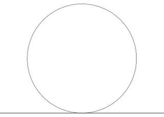
A point is in the intersection of the circle and the line if it satisfies the equations:


> onS (x,y) = x^2+(y-1)^2==1
> onL (x,y) = y==0


Notice that in R this has many solutions. In fact, we find that onS (a*d 1,0) && onL (a*d 1,0) gives True for any Float value a. Does this mean anything? Actually, it fits some people's intuition of what the intersection should look like better than the usual idea that there is only one intersection point. In fact, Protagoras argued that there was a short line segment in common between the circle and the line and that because Pythogoras's theorem gave only one solution the whole of geometry was at fault! Using R instead of the reals makes sense of this intuition. The points of the form (a*d 1,0) do, indeed, form a line tangent to the circle. In fact, there is a way to construct tangent spaces and vector fields directly from this - but instead I want to now consider Kock's construction which is slightly different.

Let D be the subset of R consisting of numbers whose square is zero. These numbers are in some sense infinitesimal. In differential geometry a vector field is intuitively thought of as an 'infinitesimal flow' on a manifold. A finite flow on a manifold, M, is simply a function f:R×M→M such that f(x,0)=0. In f(x,t) we can think of t as time and each point x on the manifold flows along a path t→f(x,t). If f is differentiable, then as t becomes smaller, the path becomes closer and closer to a short line segment which we can draw as a vector. So the intuition is that a vector field is what you get in the limit as t becomes infinitesimal. The catch is that infinitesimal things aren't first class objects in differential geometry (so to speak). You can use infinitesimals for intuition, and I suspect almost all differential geoneters do, but actually talking about them is taboo. In fact, the definition of vector field in differential geometry is a bit of a kludge to work around this issue. When most people first meet the definition of a vector field as a differential operator it comes as quite a shock. But we have no such problem. In fact, Kock defines a vector field simply as a function
f:D×M→M
such that f(0,x)=x.
In the language of SDG, a vector field is an infinitesimal flow. For example, consider


> transX d (x,y) = (x+d,y)


This simply translates along the x-axis infinitesimally. Of course this code defines a flow for non-infinitesimal values of d, but when considering this as a vector field we're only interested in when d is infinitesimal. transX defines a vector field that everywhere points along the x-axis.

For those familiar with the usual differential geometric definition of vector fields I can now make contact with that. In that context a vector field is a differential operator that acts on scalar functions on your manifold. In our case, we can think of it acting by infinitesimally dragging the manifold and then looking at what happens to the function that's dragged along. In other words, if we have a funtion, f, on the manifold, the vector field v, applied to f, is that function vf such that f (f d x)==f x + d*vf x. For example with


> h (x,y) = x^2+y^2


h (transX (d 1) (1,2)) == R 5 [2] because h(x,y)=5 and hx(x,y)=2.

I think I have enough time to briefly show how to define the Lie bracket in this context. If you have two vector fields, then intuitively you can view the Lie bracket as follows: take a point, map it using the first field by some small parameter d1, then map it using the second for time d2, then doing the first one by parameter -d1, and then the second by -d2. Typically you do not return to where you started from, but somewhere 'close'. In fact, your displacement is proportional to the product of d1 and d2. In other words, if your fields are v and w, then the Lie bracket [v,w] is defined by the equation v (-d2) $ v (-d1) $ w d2 $v d1 x==vw (d1*d2) x where vw represents [v,w]. But you might now see a problem. The way we have defined things d1*d2 is zero if d1 and d2 are infinitesimal. Kock discusses this issue and points out that in order to compute Lie brackets we need infinitesimals whose squares are zero, but whose product isn't. I could go back and hack the original definition of R to represent a new kind of algebraic structure where this is true, but in the spirit of Geometric Algebra for Free I have a trick. Consider d1=1⊗d and d2=d⊗1 in R⊗R. Clearly d12=d22=0. We also have d1d2=d⊗d≠0. And using the constructor as tensor product trick we can write:


> d1 = R (d 0) [] :: R (R Double)
> d2 = R 0 [1] :: R (R Double)


Let's test it out. Define three infinitesimal rotations:


> rotX d (x,y,z) = (x,y+d*z,z-d*y)
> rotY d (x,y,z) = (x-d*z,y,z+d*x)
> rotZ d (x,y,z) = (x+d*y,y-d*x,z)


Note that there's no need to use trig functions here. We're working with infinitesimal rotations so we can use the fact that sin d=d and cos d=1 for infinitesimal d. It is well known that [rotX,rotY]=rotZ and cyclic permutations thereof. (In fact, these are just the commutation relations for angular momentum in quantum mechanics.)

We can write


> commutator d1 d2 f g = (g (-d2) . f (-d1) . g d2 . f d1)

> test1 = commutator d1 d2 rotX rotY
> test2 = rotZ (d1*d2)


and compare values of test1 and test2 at a variety of points to see if they are equal. For example test1 (1,2,3) == test2(1,2,3). I don't know about you, but I'm completely amazed by this. We can get our hands right on things like Lie brackets with the minimum of fuss. This has many applications. An obvious one is in robot dynamics simulations where we frequently need to work with the Lie algebra of the group of rigid motions. This approach won't give us new algorithms, but it gives a very elegant way to express existing algorithms. It's also, apprently, close to Sophus Lie's original description of the Lie bracket.

I have time for one last thing. So far the only manifolds I've considered are those of the form Rn. But this stuff works perfectly well for varieties. For example, the rotations rotX, rotY and rotZ all work fine on the unit sphere. In fact, if T is the unit sphere define


> onT (x,y,z) = x^2+y^2+z^2==1


Notice how, for example, onT (rotY (d 1) (0.6,0.8,0))==True, so rotY really does give an infinitesimal flow from the unit sphere to the unit sphere, and hence a vector field on the sphere. Compare this to the complexity of the traditional definition of a vector field on a manifold.

Kock's book also describes a really beautiful definition of the differential forms in terms of infinitesimal simplices, but I've no time for that now. And I've also no time to mention the connections with intuitionistic logic and category theory making up much of his book (which is a good thing because I don't understand them).

PS The D⊗D trick, implemented in C++, is essentially what I did in my paper on photogrammetry. But there I wasn't thinking geometrically.

(I don't think I've done a very good job of writing this up. Partly I feel horribly constricted by having to paste back and forth between two text editors to get this stuff in a form suitable for blogger.com as well as periodically having to do some extra munging to make sure it is still legal literate Haskell. And diagrams - what a nightmare! So I hit the point where I couldn't face improving the text any more without climbing up the walls. What is the best solution to writing literate Haskell, with embedded equations, for a blog?)

Labels: ,

Saturday, September 16, 2006

Local and global side effects with monad transformers

There is an annual puzzle event that 90 or so people attend. Each designs a puzzle and manufactures 90 copies of it which are then shared with the other participants. All 90 then get to go home with 90 puzzles.

Anyway, an ex-coworker attends this event and I had a chance to play with his puzzle. It was one of those fitting blocks together types puzzles. It was ingeniously designed but it seemed pretty clear to me that it required a lot of combinatorial searching. So I decided to write a program in Haskell to solve it using the List monad to enable simple logic programming.

But my code had a slight problem. It worked through the puzzle and found solutions, but (1) it didn't log the steps it took to achieve those solutions and (2) I couldn't count how many combinations it searched to find the solutions. Both of these could be thought of as side-effects, so the obvious thing to do is use a monad to track these things. But there was a catch - I was already using a monad - the List monad. When that happens there's only one thing for it - using a monad transformer to combine monads.

There are two distinct ways to combine a monad with the List monad and I needed both.

Anyway, this is literate Haskell. I'll assume you're vaguely familiar with using the List monad for logic programming. I also assume you're familiar with MonadPlus though that's not something I've written about here. And I couldn't get this stuff to work in Hugs, so use ghc. Here's some code:


> import Control.Monad.List
> import Control.Monad.State
> import Control.Monad.Writer


I'm not going to describe the original puzzle now. Instead I'm going to look at an almost trivial logic problem so that we can concentrate on the monad transforming. The puzzle is this: find all the possible sums of pairs of integers, one chosen from the set {1,2} and the other from the set {2,4}, where the sum is less than 5. Here's a simple implementation.


> test1 :: [Integer]

> test1 = do
> a <- [1,2]
> b <- [2,4]
> guard $ a+b<5
> return $ a+b

> go1 = test1


Run go1 and you should get the result [3,4]. But that's just the sums. What were the pairs of integers that went into those sums? We could simply return (a,b,a+b), but in more complex problems we might want to log a complex sequence of choices and that would entail carrying all of that information around. What we'd like is to simply have some kind of log running as a side effect. For this we need the Writer monad.

If you cast your mind back, monad transformers layer up monads a bit like layers of onion skin. What we want is to wrap a List monad in a Writer monad. We do this using the WriterT monad transformer. All we have to do is add a tell line to our code, and use 'lift' to pull the items in the list monad out from one layer of onion. Here's what the code looks like:


> test2 :: WriterT [Char] [] Integer

> test2 = do
> a <- lift [1,2]
> b <- lift [2,4]
> tell ("trying "++show a++" "++show b++"\n")
> guard $ a+b<5
> return $ a+b


To get the final result we need to use runWriterT to peel the onion:


> go2 = runWriterT test2


Execute go2 and we get a list of pairs of sums and logged messages.

There's an important point to note here: we have one log per sum, so the logs are 'local'. What if we want a 'global' side effect such as a count of how many combinations were tried, regardless of whether they succeded or failed? An obvious choice of monad to count attempts is the State monad, but to make its effects 'global' we now need to make State the inner monad and make List provide the outer layer of skin. We're wrapping the opposite way to in the previous example. And now there's a catch. We use a line like a <- [1,2] to exploit the List monad. But now we no longer have a List monad, instead we have a ListT (State Integer) monad. This means that [1,2] is not an object in this monad. We can't use 'lift' either because the inner monad isn't List. We need to translate our lists into the ListT (State Integer) monad.

We can do slightly better, we can translate a list from the List monad into any other instance of MonadPlus. Remember that return x :: [X] is the same as [x] and x ++ y is the same as x `mplus` y :: [X]. For example [1,2] == (return 1) `mplus` (return 2). The latter only uses functions from the MonadPlus interface to build the list, and hence it can be used to build the equivalent of a List in any MonadPlus. To mplus a whole list we use msum leading to the definition:


> mlist :: MonadPlus m => [a] -> m a
> mlist = msum . map return


As a function [a] -> [a], mlist is just the identity. Now we're ready to go:


> test3 :: ListT (State Integer) Integer

> test3 = do
> a <- mlist [1,2]
> b <- mlist [2,4]
> lift $ modify (+1)
> guard $ a+b<5
> return $ a+b

> go3 = runState (runListT test3) 0


Run go3 to see the result. Note we had to lift the modify line because the State monad is the inner one.

And now we have one more problem to solve: bouth logging and counting simultaneously:


> test4 :: WriterT [Char] (ListT (State Integer)) Integer

> test4 = do
> a <- lift $ mlist [1,2]
> b <- lift $ mlist [2,4]
> tell ("trying "++show a++" "++show b++"\n")
> lift $ lift $ modify (+1)
> guard $ a+b<5
> return $ a+b

> go4 = runState (runListT $ runWriterT test4) 0


That's it!

We can carry out a cute twist on this. By swapping the innermost and outermost monads we get:


> test5 :: StateT Integer (ListT (Writer [Char])) Integer

> test5 = do
> a <- lift $ mlist [1,2]
> b <- lift $ mlist [2,4]
> lift $ lift $ tell ("trying "++show a++" "++show b++"\n")
> modify (+1)
> guard $ a+b<5
> return $ a+b

> go5 = runWriter $ runListT $ runStateT test5 0


go5 returns a local count of how many combinations were required for each problem, and the Writer monad now records every 'try' in one long log.

One last thing: you don't need to explicitly 'lift' things - the monad transformers have a nice interface that automatically lifts some operations. (You may need a recent Haskell distribution for this, it fails for older versions.)


> test6 :: WriterT [Char] (ListT (State Integer)) Integer

> test6 = do
> a <- mlist [1,2]
> b <- mlist [2,4]
> tell ("trying "++show a++" "++show b++"\n")
> modify (+1)
> guard $ a+b<5
> return $ a+b

> go6 = runState (runListT $ runWriterT test6) 0


It'd be cool to get rid of the mlist too. Maybe if the Haskell parser was hacked so that [1,2] didn't mean 1:2:[] but instead meant (return 1) `mplus` (return 2) like the way Gofer interprets list comprehensions in any monad. (For all I know, Gofer already does exactly what I'm suggesting.)

One thing I should add - these monad transformers really kill performance. The puzzle solver I wrote no longer gives me any solutions in the few minutes that it used to...

PS I just made up the mlist thing. There may be a better way of doing this that I don't know about. I was surprised it wasn't already in the Control.Monad library somewhere. mlist is kind of a homomorphism between MonadPlusses and I think it might make the List MonadPlus an initial object in some category or other - but that's just speculation right now.

Update: I fixed the non-htmlised <'s. I think it takes more time to convert to blogger-compatible html than to write my posts! Also take a look at this. My mlist corresponds to their liftList - and now I know I wasn't completely off the rails writing mlist.

Labels:

Friday, September 08, 2006

More Low Cost Geometric Algebra

In my second last post I showed how large algebraic structures could be built out of smaller ones using parametric polymorphism. In fact, for certain types, the type constructor acts like a tensor product in the category of algebras. It turns out that many of these structures are isomorphic to each other and Haskell provides a nice way to talk about these isomorphisms.

Before that I should say a bit more about Clifford algebras. These are an important tool in many branches of mathematics - algebraic topology, K-theory, representation theory and in theoretical physics. But one interesting aspect is that they can provide an alternative to the usual vector language of geometry. Many people will be familiar with the use of quaternions to represent 3D rotations. Clifford algebras generalise this to N-dimensions.

Before proceeding, note the footnote below on notation. And rather than write literate Haskell I've put the code here.

Back on topic: the first isomorphisms I should mention are

A⊗B≅B⊗A

for any A and B. For example HR(2)≅R(2)⊗H. As Haskell types this says that Quaternion (Matrix a) is isomorphic to Matrix (Quaternion a). Or in English: the 2×2 matrices of quaternions are isomorphic to the quaternions whose components are 2×2 matrices. This isn't completely trivial. For example let ms2sm be the isomorphism

ms2sm :: (Num a) => Matrix (Split a) -> Split (Matrix a)
ms2sm (M (S a b) (S c d) (S f g) (S h j)) =
S (M a c f h) (M b d g j)

You can see that it's a little like a matrix transpose operation.

We can draw this pictorially as:


Note that the same function, because it is polymorphic, also gives an isomorphism Matrix (Split (Quaternion a)) -> Split (Matrix (Quaternion a)). But what about the isomorphism Quaternion (Matrix (Split a)) -> Quaternion (Split (Matrix a))? We can get this almost for free using the functoriality of the constructors. The isomorphism is fmap ms2sm. We can illustrate this as:

If we implement each of the pairwise flips then in combination with fmap we can get any permutation of the constructors. And you can probably imagine some pretty braid-like diagrams describing the process. (I could mutter something about symmetric monoidal categories here.)

These isomorphisms are almost trivial - they just swap elements around. But pick up any book that discusses Clifford algebras and you'll find a bunch of extra isomorphisms listed:


CCCC

CHC(2)

HHR(4)


For example, a quaternion of quaternions is much the same as a 4×4 matrix. We choose to represent the latter as a 2×2 matrix of 2×2 entries with the isomorphism

qq2mm :: (Num a) => Quaternion (Quaternion a) -> Matrix (Matrix a)
qq2mm (Q (Q a b c d) (Q f g h j) (Q k l m n) (Q p q r s)) =
M (M (a+g+m+s) (b-f-n+r) (f-b-n+r) (a+g-m-s))
(M (c+j-k-q) (d-h+l-p) (h-d+l-p) (c+j+k+q))
(M (j-c+k-q) (d+h+l+p) (-d-h+l+p) (j-c-k+q)
(M (a-g+m-s) (-b-f+n+r) (b+f+n+r) (a-g-m+s))

(That took me a few minutes of actual work to unpack the proof of that in Spin Geometry by Lawson and Michelson so it's no longer for free!) There's a really important reason why you might want to do this. It takes 16 multiplications of the underlying elements to multiply two quaternions but it only takes 8 multiplications to multiply 2×2 matrices. A Matrix (Matrix a) can therefore be multiplied four times as fast as a Quaternion (Quaternion a). So being able to switch back and forth between repesentations is useful.

I think I now have a simple kit of parts for manipulating Clifford algebras efficiently. If I have time I should try to write a complete library for N-dimensional Clifford algebras. I wonder if I could apply it to path counting methods?

Back to isomorphisms. I want to mention two in particular. One is

Cn+8=R(16)⊗Cn


The actual isomorphism is
bott :: Num a => Quaternion (Matrix (Quaternion (Matrix a))) -> Matrix (Matrix (Matrix (Matrix a)))
bott = qq2mm . fmap mq2qm


It's prettier viewed pictorially:


As I've mentioned before, this isomorphism is an example of Bott periodicity. It pops up in many places in mathematics, for example in Supergravity or K-Theory.

This is an interesting isomorphism:

Remember that Split a is essentially a pair of objects of type a. So we can define

cliff72left,cliff72right :: Cliff7 -> Matrix (Matrix (Matrix R))
cliff72left = first . ms2sm . fmap ms2sm . (fmap (fmap ms2sm)) . qq2mm . fmap mq2qm
cliff72right = second . ms2sm . fmap ms2sm . (fmap (fmap ms2sm)) . qq2mm . fmap mq2qm

This gives not one, but two different ways to represent an element of C7 as an 8×8 matrix. But there's more to it than that. The main real-world application for quaternions is for describing rotations - they're well used in the 3D graphics world for example. Elements of C7 can be used to describe rotations in 8D. (Modulo a sign ambiguity that should be familiar to anyone who's played with quaternions.) So what he have is that a rotation in 8D can be represented with 3 different 8×8 matrices: the usual one, and the two coming from C7 (modulo the sign). This has many implications in physics. For example these three matrices describe how bosons, left-handed fermions and right-handed fermions transform under rotations. In 8-dimensions these matrices are all 8×8 making 8D a special dimension for doing physics. By a roundabout path this is closely linked to the 10D of superstring theory. This "theewayness" is known as triality which John Baez has written about a few times.


I'm getting to like this type constructor as tensor product viewpoint. I can see a lot of mathematics that be expressed nicely in it. General relativity and knot theory are two that come to mind...


Footnote about notation

I go back and forth between conventional mathematical notation and Haskell. I also have one letter abbreviations I use in function names and diagrams. The translation table is:


MathematicsHaskellAbbreviation
RRSplits
CComplexc
HQuaternionq
R(2)Matrixm
CnCliffN
C'nCliffN'

Labels: ,

Thursday, September 07, 2006

Learn Maths with Haskell

This is a quick plug for the web site of a friend of mine, David Amos. He's been working hard to produce a treasure trove of useful mathematical code in Haskell with the intention of making abstract objects more accessible to mathematics learners.


Highlights include code for


  1. Commutative algebra, including Gröbner basis computation and tools for manipulating ideals of rings.
  2. Permutation groups, including an implementation of the Schreier-Sims algorithm and tools for investigating the Rubik's cube group and its subgroups.
  3. Number theory. Includes tools for working with quadratic fields, p-adic numbers and elliptic curves, and code for factoring using Lenstra's elliptic curve algorithm.

The full repository is here. (Use that link to download the code as some of the other links appear to be broken right now.)


It'd be great to see a textbook grow out of some of this work...

Labels: ,