On writing Python one-liners.

# I'm off to the Oregon Shakespeare Festival for the weekend so no
# time to finish my Untangling series. But I do have time to post this...

# The other day someone asked me if it was possible to implement a
# certain task in one line of Python. My response was "yes, but you
# wouldn't want to." You can think of what follows as the demonstration
# that you really don't want to.

# The problem is, there are lots of Python constructions you can't
# do on one line: assigning variables, defining functions, using
# conditionals, recursion and so on. So it appears there's a limit
# to what you can do. Amazingly, all of these problems can be solved
# with the use of lambdas.

# One place you often want one line lambdas is in the use of the map
# function. So let's stick with that as an example and warm up with
# an easy example. Lets say we want to add 1 to all of the numbers
# from 0 to 19. We can write:

def inc(n):
    return n+1

print "1.",map(inc,range(0,20))

# Lambdas enable you to write that as a one-liner:

print "1.",map(lambda x:x+1,range(0,20))

# Now what happens if we want to apply a function that uses a local
# (constant) variable. For example:

def f1(n):
    m = 2*n+1
    return m+m*m

print "2.",map(f1,range(0,20))

# We can eliminate the assigment by means of a function. m changes from
# being a local to a function argument:

def f2(n):
    def g(m):
        return m+m*m
    return g(2*n+1)

print "2.",map(f2,range(0,20))

# But that seems to make things worse because now we have a function
# definition instead of a variable assigment. But we can eliminate
# that with a lambda:

def f3(n):
    return (lambda m:m+m*m)(2*n+1)

print "2.",map(f3,range(0,20))

# And now we can write the whole thing as one big lambda:

print "2.",map(lambda n:(lambda m:m+m*m)(2*n+1),range(0,20))

# But what happens if we want to define a bunch of local functions
# inside our lambda? We can use the same technique. We (1) use
# lambdas to allow us to fake local variable definitions and
# (2) use lambdas to define the functions. So we can replace this:

def f(n):
    def g(n):
        return 2*n+1

    def h(n):
        return 3*n-2

    return g(h(g(h(n))))

print "3.",map(f,range(0,20))

# with this:

print "3.",map(lambda n:(lambda g,h,n:g(h(g(h(n)))))(lambda n:2*n+1,lambda n:3*n-2,n),range(0,20))

# We're passing in lambdas as arguments to a lambda so that they
# get bound to g and h.

# But what happens if we want a recursive definition like:

def fact(n):
    if n<=1:
        return 1
    else:
        return n*fact(n-1)

print "4.",map(fact,range(0,20))

# Because the function is bound to the name fact, we can refer to
# fact by name inside the defintion of fact. How can we do this in
# a one-line lambda? We can start by eliminating the self-reference
# in a fairly standard way. First rewrite fact so it doesn't call
# itself, but calls a function passed in as an argument:

def urfact(f,n):
    if n<=1:
        return 1
    else:
        return n*f(f,n-1)

# We can then make a factorial function by calling urfact with itself,
# allowing it to carry out the recursion:

def fact1(n):
    return urfact(urfact,n)

print "4.",map(fact1,range(0,20))

# We can use urfact directly without fact1:

print "4.",map(lambda n:urfact(urfact,n),range(0,20))

# Now all we need is a one-liner definition of urfact. It's tempting to try:

def urfact1(f,n):
    return {True:1,False:n*f(f,n-1)}[n<=1]

# But that results in non-termination because it evaluates *both* branches
# of the conditional. In a lazy language like Haskell, the branch not taken
# wouldn't be evaluated. But Python can be made lazy by using...you
# guessed it...lambda. The expression lambda:x is like a lazy version
# of the expression x. It doesn't get evaluated until you apply it as a
# function of no arguments, at which time it takes on the value x. So we
# can rewrite urfact as:

def urfact2(f,n):
    return {True:lambda:1,False:lambda:n*f(f,n-1)}[n<=1]()

# And we get

print "4.",map(lambda n:urfact2(urfact2,n),range(0,20))

# Note how we use urfact2 twice, so we need the trick above for local
# definitions to get it down to one reference:

print "4.",map(lambda n:(lambda f:f(f,n))(urfact2),range(0,20))

# And now we can replace urfact2 with a lambda

print "4.",map(lambda n:(lambda f:f(f,n))(lambda f,n:{True:lambda:1,False:lambda:n*f(f,n-1)}[n<=1]()),range(0,20))

# And that's enough for now. I expect that if we keep going we'll find 
# way to rewrite any Python program as a one liner. You could probably
# even write a program to automatically 'compile' a usable subset of
# Python into one liners.

# But you probably don't want to do that.

Untangling with Continued Fractions: Part 4

> {-# LANGUAGE MultiParamTypeClasses,FunctionalDependencies,FlexibleInstances,GeneralizedNewtypeDeriving #-}

> module Main where

> import Test.QuickCheck
> import qualified Data.Map as M
> import Control.Monad
> import Ratio

> infixl 5 .+
> infixl 6 .*

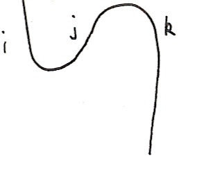
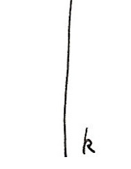
As I've mentioned previously, we need to choose values for our pieces of knot or tangle so that when they're combined together we get something that tells us about the knot or tangle, not the diagram. For example, suppose our diagram contains this piece:

That piece is isotopic to:

We want any kind of evaluation of our diagram to be independent of which one of these we've chosen. In other words, among other things we need this function:

> cupcap i = do
>   (j,k) <- cap
>   cup (i,j)
>   return k

to equal this function:

> straight i = do
>   return i

I've already said how in the vector space monad, these correspond to summations, so really we want these two expressions to be equal (using the summation convention):

M^ijN_jk=δⁱ_k

(δⁱ_k is 1 if i=k and zero otherwise, ie. the identity matrix.)
The left hand side is just the rule for multiplying matrices. So we require M to be the inverse of N.

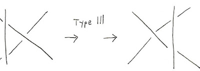
Now we can start on some real knot theory. There is a collection of 'moves' we can perform on a diagram called Reidemeister moves. Here are diagrams illustrating them:




There are three types of move that we call type I, type II and type III.

These diagrams are intended to show changes we can make to a part of a bigger knot or tangle. It's not hard to see that these are isotopies, they're just simple operations we can perform on a knot or tangle by moving the string a little bit. If you perform one of these moves on a knot or tangle then you should end up with merely a different diagram representing the same knot or tangle. Each of these corresponds to an equality of monadic expression, or an equality of summations. But the really important part is that these are all you need to consider. Every isotopy can be constructed out of these moves. So if we can satisfy the corresponding equalities of expressions then we automatically have a knot invariant that tells us about the underlying knot or tangle, not just the diagram.

Unfortunately, there's a catch. Satisfying the equality for a type I move is too onerous. So we'll just concentrate on type II and III. But the good news is that it doesn't matter, there are workarounds.

Let a be an unknown complex number. We're going to build expressions from a but they're all going to be polynomials in a and its reciprocal, like a+a^2-3/a. These are known as Laurent polynomials and I pointed out recently that I can use the Group type class to represent them.

> i = 0 :+ 1
> newtype Z = Z Int deriving (Eq,Ord,Show,Num)
> type Poly = V (Complex Rational) Z

In other words, elements of Poly are weighted linear combinations of integers. We can think of each integer n as representing aⁿ and the weights being coefficients of these powers. Amazingly the group multiplication multiplies these things out correctly.

a and ia represent a and a^-1.

> a = return (Z 1) :: Poly
> ia = return (Z (-1)) :: Poly

We can now satisfy the type II and III Reidemeister moves with these definitions:

> cup :: (Bool,Bool) -> V Poly ()
> cup (u,v) = case (u,v) of
>   (False,True) -> (-i .* ia) .* return ()
>   (True,False) -> (i .* a) .* return ()
>   otherwise -> zero

> cap :: V Poly (Bool,Bool)
> cap = (-i .* ia) .* return (False,True) .+ (i .* a) .* return (True,False)

> over :: (Bool,Bool) -> V Poly (Bool,Bool)
> over (u,v) = a .* do
>   () <- cup (u,v)
>   cap
>   .+
>   ia .* return (u,v)

> under :: (Bool,Bool) -> V Poly (Bool,Bool)
> under (u,v) = ia .* do
>   () <- cup (u,v)
>   cap
>   .+
>   a .* return (u,v)

(I'm making the V monad do double duty here. I'm using it to represent the Laurent polynomials, but I'm also using it to represent vectors over the Laurent polynomials.)

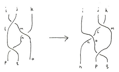
For example, here's what a type III move looks like if we try to arrange things nicely in terms of our standard 'components':

That gives rise to the two functions

> left (i,j,k) = do
>   (l,m) <- under (i,j)
>   (n,o) <- over (m,k)
>   (p,q) <- over (l,n)
>   return (p,q,o)

and

> right (i,j,k) = do
>   (l,m) <- over (j,k)
>   (n,o) <- over (i,l)
>   (p,q) <- under (o,m)
>   return (n,p,q)

whose equality can be tested with

> test1 = quickCheck $ \(x,y,z) -> left (x,y,z)==right (x,y,z)

I'll leave checking the type II rule as an exercise.

With these defintions we can take any knot diagram and compute a value for it. Note that because a not has no loose ends we have no inputs and no outputs so the result won't be a function but a value, a polynomial in a and its reciprocal. This is known as the Bracket Polynomial.

As mentioned above, the bracket polynomial fails to be a knot invariant. Two diagrams related by type I moves will have different bracket polynomials. With a little bit of sleight of hand we can apply a fudge factor to l with those extra loops and we end up with the Jones polynomial. As that's not my main goal here, I'll let you read how to use the writhe get from the bracket polynomial to the Jones polynomial at Wikipedia. But do I want to make another digression.

It's tricky to define knot invariants. The problems is that knots are topologically invariant in the sense that you can deform a knot in lots of ways and it's still the same knot. This rules out most attempts at using the geometry of a knot to define an invariant. Just about any geometrical feature you find in a particular configuration will be ruined by deforming the knot. But here's an idea: suppose you could compute some geometrical property from a particular curve representing a knot and then find the average of that value for all possible curves representing the same knot. Then we'd get a knot invariant as it wouldn't depend on a particular choice of representative curve. But there's a catch. We need to average over an infinite space, the space of all curves representing a knot. On the other hand, there is a perfectly good tool for averaging over infinite sets: integration. But there's another catch: the space of all curves representing a knot is very large, infinite dimensional in fact, and we don't have very good theory for how to do this. At least mathematicians don't. But physicists integrate over spaces of paths all the time, ever since Feynman came up with the path integral. Amazingly, Ed Witten showed that tere was already a physical model that fit the bill: Chern-Simons theory. In fact, Witten showed that the Jones polynomial, which as I've already mentioned came originally out of statistical mechanics, could be derived from this theory.

Anyway, enough of that digression. In the next installment I'll show how the above can be modified for use with tangles and give my final algorithm.


In the last installment (I think) I'll show how we can derive the rational number for a tangle using the bracket polynomial.

---

The following is the 'library' behind the code above. Most of it is simply built up from what I've said in recent weeks.

> swap (x,y) = (y,x)

> class Num k => VectorSpace k v | v -> k where
>     zero :: v
>     (.+) :: v -> v -> v
>     (.*) :: k -> v -> v
>     (.-) :: v -> v -> v
>     v1 .- v2 = v1 .+ ((-1).*v2)

> data V k a = V { unV :: [(k,a)] } deriving (Show)

> reduce x = filter ((/=0) . fst) $ fmap swap $ M.toList $ M.fromListWith (+) $ fmap swap $ x

> instance (Ord a,Num k) => Eq (V k a) where
>   V x==V y = reduce x==reduce y

> instance (Ord a,Num k,Ord k) => Ord (V k a) where
>   compare (V x) (V y) = compare (reduce x) (reduce y)

> instance Num k => Functor (V k) where
>     fmap f (V as) = V $ map (\(k,a) -> (k,f a)) as

> instance Num k => Monad (V k) where
>     return a = V [(1,a)]
>     x >>= f = join (fmap f x)
>         where join x = V $ concat $ fmap (uncurry scale) $ unV $ fmap unV x
>               scale k1 as = map (\(k2,a) -> (k1*k2,a)) as

> instance Num r => MonadPlus (V r) where
>     mzero = V []
>     mplus (V x) (V y) = V (x++y)

> instance (Num k,Ord a) => VectorSpace k (V k a) where
>     zero = V []
>     V x .+ V y = V (x ++ y)
>     (.*) k = (>>= (\a -> V [(k,a)]))

> e = return :: Num k => a -> V k a
> coefficient b (V bs) = maybe 0 id (lookup b (map swap (reduce bs)))

> diag a = (a,a)
> both f g (a,b) = (f a,g b)

> class Group m a where
>     unit :: () -> m a
>     counit :: a -> m ()
>     mult :: (a,a) -> m a
>     comult :: a -> m (a,a)
>     anti :: a -> m a

> instance Monad m => Group m Z where
>     unit _ = return (Z 0)
>     counit _ = return ()
>     mult = return . uncurry (+)
>     comult = return . diag
>     anti = return . negate

> newtype Identity a = I a deriving (Eq,Ord,Show)

> instance Monad Identity where
>     return x = I x
>     I x >>= f = f x

> data K = K Rational Rational deriving (Eq,Show)

> instance Num K where
>   K a b + K a' b' = K (a+a') (b+b')
>   K a b * K a' b' = K (a*a'+2*b*b') (a*b'+a'*b)
>   negate (K a b) = K (negate a) (negate b)
>   abs _ = error ""
>   signum _ = error ""
>   fromInteger i = K (fromInteger i) 0

> instance Num k => Num (V k Z) where
>   a + b = a .+ b
>   a * b = do
>       u <- a
>       v <- b
>       mult (u,v)
>   negate a = (-1) .* a
>   fromInteger n = fromInteger n .* return 0
>   abs a = error ""
>   signum a = error ""

> data Complex a = (:+) { realPart :: a, imagPart :: a } deriving (Eq,Show)

> instance Num a => Num (Complex a) where
>   (a :+ b) + (a' :+ b') = (a+a') :+ (b+b')
>   (a :+ b) * (a' :+ b') = (a*a'-b*b') :+ (a*b'+a'*b)
>   negate (a :+ b) = (-a) :+ (-b)
>   fromInteger n = fromInteger n :+ 0
>   abs (a :+ b) = undefined
>   signum (a :+ b) = undefined

> instance Fractional a => Fractional (Complex a) where
>   recip (a :+ b) = let r = recip (a*a+b*b) in ((a*r) :+ (-b*r))
>   fromRational q = fromRational q :+ 0

> instance Ord (Complex Float) where
>   compare (a :+ b) (c :+ d) = compare (a,b) (c,d)

Two Papers and a Presentation

I've been slow to write the last couple of parts on my untangling series as I've been pretty busy lately. Among other things I've finally got around to submitting a couple of graphics related papers (that I actually wrote ages ago) for publication. Not sure they'll get accepted but there's no harm trying. I'll probably write blog posts about these in the near future now that I have permission from my employer to talk about them.

Note: Neither of these are anything I actually use at work. Well, I've used the adjoint one a tiny bit. The latter is in the spirit of computational geometry papers: it demonstrates an algorithm that runs (asymptotically) in the fastest possible time, but in practice you'll probably want to use an approximation that looks just as good. I was amazed I was able to find a practical application for a result that came out of toric varieties, but it's going to be tough on the reviewers as there seem to be so few people in the graphics world who know about multidimensional DSP techniques.

Two Tricks for the
Price of One: Linear Filters and their Adjoints

Fast and Exact
Convolution with Polygonal Filters

Of course, straight after submitting I noticed a bunch of pieces missing from some expressions. In places designed to help disambiguate things for the reviewers as well. Ho hum.

I also recently presented a very short presentation at the "Stupid Rat Tricks" part of the Renderman User Group: quine.sl: a self-shading shader. (For more on RSL see Wikipedia.) The source is available here. I don't think the company lawyers fully appreciated that this shader now allows their handiwork to be used like a texture map.

My presentation was completely blown away by the guy who implemented a large part of the Renderman interface completely in bourne shell. I can't think of a stupider thing than that! :-)

Back to untangling in the next post.

Update: I added a Mathematica 5 notebook illustrating the transfer functions in the polygonal filter paper.