Search This Blog

Wednesday, December 27, 2006

Tying Knots Generically

A comment by a friend and a puzzle on Lambda the Ultimate made me realise that the function loeb that I defined a few weeks back does have a nice application.


> import Maybe
> import Data.Map

> loeb :: Functor a => a (a x -> x) -> a x
> loeb x = fmap (\a -> a (loeb x)) x


The problem it helps to solve is this: building circular datastructures in Haskell, otherwise known as Tying the Knot. loeb solves this problem in a very generic way that imposes the minimum of restrictions on the user.

Remember how in my previous article I showed how you could view loeb as a kind of spreadsheet evaluator. You have a container of functions and that is converted into another container by applying these functions to the final container. This is a circular definition, we're applying the functions to the final result to get the final result. If we think of the final container as a collection of answers to a bunch of problems, loeb allows each element to be constructed using references to any of the other answers in the container, even if they haven't actually been found yet. This is exactly what we need to make circular references.

Firstly, let's look at doing something similar to the Tying the Knot web page to solve Derek's puzzle. Here potential links are made by using a dictionary structure to allow names of objects to stand for direct references to objects. So define an operator to perform pointwise concatenation of string-valued functions:


> f +++ g = \x -> f x ++ g x


Now define lookup into the dictionary, substituting a default value if needed:

And now we can translate some example equations into Haskell by hand. I'm considering define a x *b and define b y *a. Note how it's trivial to write a parser to make these objects because there's nothing circular going on:


> equations = fromList
> [
> ("a",const "x"+++lookup "b"),
> ("b",const "y"+++lookup "a")
> ] where lookup = Data.Map.findWithDefault ""


We now just apply loeb to get a dictionary containing the actual values:


> values = loeb equations
> a = fromJust $ Data.Map.lookup "a" values


We can use a similar method to make a doubly linked list. Here is "A", "B" and "C" in a list with each letter pointing to its predecessor and successor if it exists:


> data DList a = Nil | Node a (DList a) (DList a) deriving Show
>
> val (Node a _ _) = a
> rt (Node _ _ r) = r
> lft (Node _ l _) = l
>
> nodes = fromList
> [
> ("a", \d -> Node "A" Nil (lookup "b" d)),
> ("b", \d -> Node "B" (lookup "a" d) (lookup "c" d)),
> ("c", \d -> Node "C" (lookup "b" d) Nil)
> ] where lookup = Data.Map.findWithDefault Nil
>
> abc = loeb nodes
> b = fromJust $ Data.Map.lookup "b" abc


b is now a doubly linked list and we can use lft and rt to walk up and down it.

And here's a nice advantage of using loeb. You don't have to restrict yourself to storing information about links in a dictionary. Any functorial container will do. For example here's a doubly linked circular list of the integers from 0 to 99 made without using any names:


> zlist = [\z -> Node i (z!!((i-1) `mod` 100)) (z!!((i+1) `mod` 100)) | i <- [0..99]]
> z = loeb zlist


Note how working your way up and down zlist is a slow process because you need to use the slow (!!) to access elements. But stepping up and down any element of z takes time O(1). Potentially very useful!

But there is a slight problem with loeb. I'd like to be able to handle errors better and the obvious way to do that is by allowing the use of monads to handle exceptions, for example if a name lookup in a dictionary fails. I attempted to do this as follows:


> class Monad m => MFunctor m f where
> fmapM :: (a -> m b) -> f a -> m (f b)

> instance Monad m => MFunctor m [] where
> fmapM = mapM

> loebM :: (Monad m,MFunctor m a) => a (a x -> m x) -> m (a x)
> loebM x = r where
> r = do
> lx <- r
> fmapM (\a -> a lx) x

> u = loebM [const (Just 1),const (Just 2)]


But attempting to evaluate u overfows the stack. It also failed when I tried modifying it to use MonadFix. So here's a puzzle. Can you write a monadic version of loeb? It seems like something that would be very useful for writing interpreters for programming languages that allow mutually recursive definitions.

So my original intuition a few weeks back was right. Taking an interesting axiom of modal logic, interpreting as a type, and them finding an implementation, did lead to something useful.


By the way, while I was thinking about loeb I was led to consider what I call tautological containers. These are containers where each element tells you how to extricate it from the container. For example, these can be thought of as tautological: (fst,snd), [head,head.tail], [(!!n) | n <- [0..]] and [("a",fromJust . lookup "a"),("b",fromJust . lookup "b")]. Can you see any use for these objects? Are they universal for some category diagram? I have partial answers to these questions but maybe you can make more sense of them than me.


Update: Ocaml version by Matias Giovannini.

Tuesday, December 19, 2006

Evaluating cellular automata is comonadic

Paul Potts's post inspired me to say something about cellular automata too.

So here's the deal: whenever you see large datastructures pieced together from lots of small but similar computations there's a good chance that we're dealing with a comonad. In cellular automata we compute the value of each cell in the next generation by performing a local computation based on the neighbourhood of that cell. So cellular automata look like they might form a good candidate for comonadic evaluation.

I want to work on 'universes' that extend to infinity in both directions. And I want this universe to be constructed lazily on demand. One way of doing that is to represent a 'universe' as a centre point, a list of all elements to the left of that centre point and a list of all elements to the right. Here's a suitable
type:


> data U x = U [x] x [x]


For example U [-1,-2..] 0 [1,2..] can be thought of as representing all of the integers in sequence.

But this actually contains slightly more information than a list that extends to infinity both ways. The centre point forms a kind of focus of attention. We could shift that focus of attention left or right. For example consider

U [-2,-3..] (-1) [0,1..]

This represents the same sequence of integers but the focus has been shifted left. So think of the type U x as being a doubly infinite sequence with a cursor. (In fact, this makes it a kind of zipper.)

We can formalise the notion of shifting left and right as follows:


> right (U a b (c:cs)) = U (b:a) c cs
> left (U (a:as) b c) = U as a (b:c)


An object of type U is semantically like a C pointer into a const block of memory. You can increment it, decrement it and dereference it using the function I'll call coreturn below.

As U is a kind of list structure, it needs a map. In fact, we can define fmap for it:


> instance Functor U where
> fmap f (U a b c) = U (map f a) (f b) (map f c)


Now the fun starts. First I'll bemoan the fact that Comonads aren't in the standard Haskell libraries (at least I don't think they are). So I have to define them myself:


> class Functor w => Comonad w where
> (=>>) :: w a -> (w a -> b) -> w b
> coreturn :: w a -> a
> cojoin :: w a -> w (w a)
> x =>> f = fmap f (cojoin x)


cojoin is the dual to the usual join function. I've chosen to do things the category theoretical way and define =>> in terms of cojoin.

And here's why U forms a Comonad:


> instance Comonad U where
> cojoin a = U (tail $ iterate left a) a (tail $ iterate right a)
> coreturn (U _ b _) = b


Look closely at cojoin. It turns a into a 'universe' of 'universes' where each element is a copy of a shifted left or right a number of times. This is where all the work is happening. The reason we want to do this is as follows: we want to write rules that work on the local neighbourhoods of our universe. We can think of a universe with the cursor pointing at a particular element as being an element with a neighbourhood on each side. For example, we can write a cellular automaton rule like this:


> rule (U (a:_) b (c:_)) = not (a && b && not c || (a==b))


In order to apply this everywhere in the universe we need to apply the rule to each possible shift of the universe. And that's what cojoin does, it constructs a universe of all possible shifts of a. Compare with what I said here. So believe it or not, we've already written the code to evaluate cellular automata. u =>> rule applies the rule to u. The rest is just boring IO:


> shift i u = (iterate (if i<0 then left else right) u) !! abs i
>
> toList i j u = take (j-i) $ half $ shift i u where
> half (U _ b c) = [b] ++ c
>
> test = let u = U (repeat False) True (repeat False)
> in putStr $
> unlines $
> take 20 $
> map (map (\x -> if x then '#' else ' ') . toList (-20) 20) $
> iterate (=>> rule) u


Lazy infinite structures, comonads, zippers. I think I'm just beginning to get the hang of this functional programming lark! Over Xmas I might feel ready to try writing a piece of code longer than a dozen or so lines.

Anyway, I must end with a credit. I probably wouldn't have come up with this if I hadn't read this paper by Uustalu and Vene.

Wednesday, December 13, 2006

Why isn't ListT [] a monad?

Well I'm back from my vacation. But this isn't my personal blog so I think it's time to dive right in. Anything to take my mind off these mosquito bites...

So consider the free semiring R generated by some set S. In other words, S consists of finite sums and products of 0, 1 and elements of S and where the only simplification rules allowed are

a+0=a, a+b=b+a, a+(b+c)=(a+b)+c

a1=1, a(bc) = (ab)c

a(b+c) = ab+ac and (a+b)c = ac+bc.


For example, consider a term like ab+c(ef+gh). We can use distributivity to multiply this out to ab+cef+cgh. There's not much else we can do to simplify this. Now notice that if you multiply out all of the brackets wherever you can, ie. use distributivity until you can no longer, you end up with an expression that is a sum of terms and each term is a product of generators from S. (The sum of terms may be empty, in which case it's zero, and each of the terms may be a product of zero generators, in which case it is 1). This allows us to write elements of R in a canonical form: as a set of terms where each term is an ordered list of generators. For example, we could write ab+cef+cgh as {[a,b],[c,e,f],[c,g,h]}. Notice how the commutativity of addition is represented by the fact that we're using a set of terms, but each term is a list of generators because we're making no assumption about the commutativity of multiplication.

In Haskell it's more convenient to work with lists. Se we'll represent our running example as [['a','b'],['c','e','f'],['c','g','h']]. So if S is the Haskell type corresponding to our set of generators, then [[S]] can be thought of as the free semiring generated by elements of S, with the proviso that we consider two elements equal if one can be reordered to the other. Note that []=0 and [[]] = 1.

Now suppose that S is itself a free semiring generated by T. Then R = [[ [[T]] ]], modulo ordering. If you think about it, there's a nice way to use the algebraic structure to 'flatten' an element of [[ [[T]] ]] down to an element of [[T]]. R is freely generated by elements of S, in other words it consists of sums of products of elements of S. But the elements of S are themselves sums and products. So we have sums of products of sums of products. I emphasised two words in that sentence. This is because R contains subparts that are products of sums. If we multiply these out in the usual way, we get sums of sums of products of products. Group the sums and products together, and we get back to sums of products. Here's an example: any element of T trivially gives an element of S. So if a,b,c,e,f,g and h are all in T, then a,b,c and ef+gh are all in S and hence are generators of R, so ab+c(ef+gh) is in R. Multiply out and we obviously have the element ab+cef+cgh of S. It's not hard to see how this generalises to map any element of S back down to T. So we have maps


T -> [[T]] (by trivial inclusion of generators)

[[ [[T]] ]] -> [[T]] (by above argument)


Look to you like a monad? Of course it does! :-) But what monad is it?

First, let's implement the map [[ [[T]] ]] -> [[T]]. After tinkering I came up with


> import Control.Monad.List

> flatten x = concatMap (map concat . sequence) x


We can test it out


> x = [[ [['a']],[['b']] ], [ [['c']],[['e','f'],['g','h']] ]]
> test1 = flatten x


It multiplies out exactly the way we want.

Now compare with running this:


> x' = ListT [[ ListT [['a']],ListT [['b']] ],
> [ ListT [['c']],ListT [['e','f'],['g','h']] ]]
> test2 = runListT $ join x'


In other words, apart from the ListT fluff, join for ListT [] is flatten. So if we consider lists as a mechanism to represent sets, ListT [] is revealed as the monad of semirings. I'm not sure, but I think that historically this is where monads originally came from. Certainly there are many papers on the relationship between monads and algebraic structures like semirings.

And now I can answer my original question. In a semiring, addition is commutative, so the order of terms doesn't matter. But in ListT [], we're using lists, and order does matter in a list. So if we do take order into account, then really ListT [] is the monad of semirings where both addition and multiplication is non-commutative. And here's the problem: in general, there is no such thing as a freely generated semiring with non-commutative addition.

Here's why: consider the expression ((a+b)+(a+b))*((a+b)+(a+b)). Multiply out the inner parentheses first and we get

(a+b+a+b)*(a+b+a+b)

= a*a+a*b+a*a+a*b+…


Now multiply out the outer parentheses first and we get

(a+b)*(a+b)+(a+b)*(a+b)+(a+b)*(a+b)+(a+b)*(a+b)

= a*a+a*b+b*a+b*b+…


The terms are coming out in a different order. Essentially distributivity doesn't work in a semiring with non-commutative addition.

This translates directly into failure of one of the monad laws. First write our expression as an object of type ListT []:

u = a+b

> u = ListT [["a"],["b"]]


v = (a+b)+(a+b)

> v = ListT [[u],[u]]


w = ((a+b)+(a+b))*((a+b)*(a+b))

> w = ListT [[v,v]]


join multiplies out parentheses. So working from the outer parentheses inwards we can use:


> expanded1 = join $ join w
> go1 = runListT expanded1


Working outwards from the inner parentheses we get:

> expanded2 = join $ fmap join w
> go2 = runListT expanded2


(Note how I use fmap to 'duck down' through the outer layer of parentheses so as to multiply out each of the subexpressions first.)

Evaluate go1 and go2 and you'll see that they corresponds to the two ways of multiplying out that I gave above. And more importantly, the values of expanded1 and expanded2 aren't equal, meaning that join . join = join . fmap join isn't satisfied. You may recognise this: it's one of the monad laws. (At least it's one of the monad laws written the way category theorists write them.) So we ain't got no monad.


I think this is now a fairly complete analysis of what ListT [] is all about. So one obvious remaining question is: where do games come into all this? The answer is that games form a semiring in a way that I haven't seen documented anywhere (though is surely common knowledge). I'd explain but I've run out of time...

Note that the reason ListT [] isn't a monad is that [] isn't commutative, in some sense. This has been observed many times in the past. Two papers mentioning this are this and this.

I actually figured out all of this stuff before this. I realised that the trees I was scribbling on the backs of my envelopes to represent elements of semirings could actually be generalised to just about any kind of tree, so I wrote about the general case first.

I prefer my example of ListT [] failing to be a monad to the examples given here. The latter make use of the IO monad so they aren't quite as 'pure'.

Saturday, December 02, 2006

A Yonedic Addendum

Firstly, blogger.com seems to have temporarily lost the preview feature so I'm writing this as blind HTML. I won't know exactly how it looks until I hit 'publish'. (It's not real HTML so it's no good just pasting into a web page.)

I kept meaning to follow up on my earlier post about the Yoneda lemma by working out if each of the three examples I considered were Theorems for Free! But it's tedious work to decrypt the free theorem as it is generated by the procedure in Wadler's paper. But then I suddenly realised that lambdabot could do the work for me. I looked at all three examples that I gave, but I'll just spell out the details for the last one here. Consider machines of type forall b. (A -> b) -> C -> b. What free theorem do we get from that? If you don't have lambdabot you can see here. But first I need to point out either a limitation in that free theorem prover, or a limitation of my understanding of it. It seems to attach a forall for every free variable. But I want to have A and C fixed, but unknown. It makes a difference. In the end a cheated by considering the type


(Float -> b) -> Char -> b


The free theorem is
h1 (f1 x2) = g1 x2) => h1 (t1 f1 x1) = t1 g1 x1

where t1 :: forall b. (Float -> b) -> Char -> b. With a tiny bit of work we can deduce

t1 h1 = h1 . t1 id.


Using my earlier notation, that is essentially check3 . uncheck3 = id. Similar results followed for the other examples. So I conjecture that for functors F, the free theorems for (a -> b) -> F b are just proofs of the Yoneda lemma (well, the less trivial direction at least). I'm guessing this is all blindingly obvious to type theorists but it's all new to me.


Anyway, a couple of thoughts come to mind. This stuff is all about parametricty, and part of what makes this work is that any polymorphic function (with the same restrictions in Theorems for Free!) that looks like a natural transformation is a natural transformation in the category of Haskell types. But Theorems for Free! also talks about functions that don't look like natural transformations. For example consider the type (a->a)->(a->a). The free theorem reflects the fact that any such function must simply raise its argument to some non-negative integer power. But it seems to me that when the free theorem is written in point-free style, then functions (ie. functions that map objects to arrows like the way natural transformations do) in a general category that satisfy this theorem are also in some sense 'natural'. So is there a wider sense of 'natural' in a category that I should know about?


What I find interesting here isn't necessarily the type theory in itself. What I think is interesting is that the type theory provides nice intuition for other applications for the Yoneda lemma, and indeed other parts of category theory. Up to now, my spare time reading of computer science hasn't really fed back back into my understanding of other branches of mathematics. But this time it has. Even though the category of Haskell types and functions looks a lot like Set, it has nice properties of its own that deepen your understanding of categories in general.


Anyway, while I'm on the subject of things Yonedic, here's an application of category theory to the composition of music. The author s claim the Yoneda lemma has applications in this field. Yes, you read that correctly. No, it's not April 1. In fact, I discovered this by doing a google code search on yoneda.


One last thing. I should credit augustss for getting me to think about the mathematical significance of parametricity in the first place. That was 6 months ago. Trying to do mathematics when you only have a couple of hours free a week is slow going.


BTW I'm in Mexico on vacation for the next week and a half. On the plane I'll be reading (at least) the papers on cake cutting and Venn diagrams mentioned here: Ars Mathematica.


Friday, November 24, 2006

How Telescopes Really Work and What You Can See Through Them

For my birthday a few weeks ago (40!) I received an 8" dobsonian telescope from my wife and her family. Of course the weather here in Northern California suddenly took a turn for the worse immediately after I brought it home, but there have still been a few clear nights.

One of the frustrating things about astronomy is that what you can see with an amateur telescope from your back yard in a well lit city is quite different from what you can see from the wilderness with a telescope the size of a truck. Unfortunately, even a great book like The Backyard Astronomer's Guide is dominated by the latter type of picture (like that fantasic picture of the Andromeda galaxy on its cover). So I thought I'd tell it like it really is and give you an idea of what you can see from my location.

How Telescopes Work


Before that, I want to mention something about telescopes. My telescope is a Newtonian reflector and if you look at the pictures on Wikipedia you'll notice that the secondary mirror forms an obstruction that blocks some of the light entering the telescope. A frequently asked question is "why can't you see the obstruction through the scope"? In fact, if you put your hand in front of the aperture the effect on what you see, if the image is in focus, is negligible, just a little darkening. The explanation is very simple, but nobody seems to phrase it the same as me.

The idea is this: a lens, that's in focus, is a device that converts direction into position. Suppose the telescope is oriented along the x-axis. Think of a ray of light as having the equation y=mx+c. Think of m as the ray direction and c as its position. If that ray passes through a lens or mirror and is projected onto a screen, denote the position at which it arrives on the screen by f(m,c). It's clearly a function of m and c. The crucial point is that for a screen at precisely the focal length away from the lens or mirror, f(m,c) is independent of c. That's the raison d'être of a telescope. All rays with gradient m arrive at the same point. So we end up with a bright image because we can collect lots of rays coming from the same direction. But also, any information about the ray's position, ie. c, has been erased. Information about the shape of the obstruction is positional information contained in c. This has been erased, and hence you can't see the obstruction. In practice you really need to consider primary lens (or mirror), plus eyepiece, plus lens of the eye projecting onto the retina, but the principle is the same. For the more formally inclined, the erasure of c information corresponds to a zero in a transfer matrix.

In brief: a lens or mirror focussed on infinity is a position eraser.

And What You Can See Through Them


Andromeda Galaxy


My first two subjects were probably the same as every other amateur astronomer. I started with the Andromeda galaxy. Through binoculars it looks like a faint fuzzy blob. And here's the truth of how it looks through a telescope: it looks like a fuzzy blob, at least from a well lit city. I couldn't make out any kind of structure at all, let alone spiral arms. It didn't even look elliptical, just a circular blob with brightness falling off radially from the centre. I also saw one of its neighbours, M32 or M110. At first I thought that the fuzzy blob was the galaxy and that I needed more magnification to see detail. But now I think that I was seeing just the core of the Andromeda galaxy with the arms filling a wider area but remaining invisible because they're no brighter that the sky in my part of the world.

Orion Nebula


The Orion nebula, on the other hand, was stunning! In outline, it looked remarkably like the picture at wikipedia, but without the colour. When I switched to using a filter (a narrow bandpass Lumicon UHC filter) it became even clearer. Not only could I clearly see the shape of the nebula but I could also see structure all the way through the cloud. It looked even better after I'd been viewing it for a while, probably as my eyes became better adapted to the dark. This was the best thing I've seen through a telescope ever!

Almach


I'll mention the last thing I looked at: γ Andromedae, otherwise known as Almach. It's a binary star system that can't be resolved with the naked eye. I used a wide field of view lens and was disappointed to see that it still looked like a single star. But then I switched eyepieces and I saw it - a beautiful pair of stars, one brighter and yellowy orange and the other deep blue. You read about the colour of stars but it's often a disappointment. A single star on its own tends to look white with a hint of colour because the eye doesn't register colour well in such low light conditions. But when you see two contrasting stars so close together it makes a world of difference. The deep blue of the smaller star was unmistakable and the blue really was astonishingly blue. That must be quite a sight for the γ Andromedans. But I should add that the blue star is in fact a triple star system in its own right, so γ Andromedae is actually a quadruple star system. I was unable to resolve more stars than two (and you can only tell there are four by inference from spectrography, not direct viewing).

I also tried to find the Crab Nebula. I'm 99% sure that I was pointing at the right part of the sky and I did in fact see a faint smudge just at the limits of my perception. I had a jiggle the telescope around a bit just to be sure I wasn't imagining it, but sure enough, it appeared to be attached to the sky, not the scope or my eyes. But it certainly didn't look like the pictures.

Anyway, now you have a better idea of what you can see from a city.

Monday, November 20, 2006

From Löb's Theorem to Spreadsheet Evaluation

> import Control.Monad.Reader

I've run 3 miles, the Thanksgiving turkey's in the oven, now I just need to do something impossible before I can have breakfast.

As I've mentioned in the past, sometimes you can write useful Haskell code merely by writing something that type checks successfully. Often there's only one way to write the code to have the correct type. Going one step further: the Curry-Howard isomorphism says that logical propositions corresponds to types. So here's a way to write code: pick a theorem, find the corresponding type, and find a function of that type.

One area that seems fruitful for this approach is modal logic. The axioms of various modal logics correspond to the types of familiar objects in Haskell. For example the distribution axiom:

□(a→b)→(□a→□b)

Looks just like the type of ap :: (Monad m) => m (a -> b) -> m a -> m b.

So I'm looking at the books on my shelf and there's The Logic of Provability by Boolos. It's about a kind of modal logic called provability logic in which □a roughly means "a is provable". One of the axioms of this logic is a theorem known as Löb's theorem.

Before getting onto Löb's Theorem, I should mention Curry's Paradox. (Before today I didn't know Haskell Curry had a paradox associated with his name - though I've met the paradox itself before as it got me into trouble at (high) school once...) It goes like this:

Let S be the proposition "If S is true, Santa Claus exists".

Suppose

S is true.

Then

If S is true, Santa Claus exists.

So, still assuming our hypothesis, we have

S is true and if S is true, Santa Claus exists.

And hence

Santa Claus exists.

In other words, assuming S is true, it follows that Santa Claus
exists. In otherwords, we have proved

If S is true then Santa Claus exists

regardless of the hypothesis.
But that's just a restatement of S so we have proved

S is true

and hence that

Santa Claus exists.


Fortunately we can't turn this into a rigorous mathematical proof though we can try, and see where it fails. In order to talk about whether or not a proposition is true we have to use some kind of Gödel numbering scheme to turn propositions into numbers and then if a proposition has number g, we need a function True so that True(g)=1 if g is the Gödel number of something true and 0 otherwise. But because of Tarski's proof of the indefinability of truth, we can't do this (to be honest, the argument above should be enough to convince you of this, unless you believe in Santa). On the other hand, we can replace True with Provable, just like in Gödel's incompleteness theorems, because provability is just a statement about deriving strings from strings using rewrite rules. If we do this, the above argument (after some work) turns into a valid proof - in fact, a proof of Löb's theorem. Informally it says that if it is provable that "P is provable implies P" then P is provable. We did something similar above with P="Santa Claus exists". In other words

□(□P→P)→□P.


So I'm going to take that as my theorem from which I'll derive a type. But what should □ become in Haskell? Let's take the easy option, we'll defer that decision until later and assume as little as possible. Let's represent □ by a type that is a Functor. The defining property of a functor corresponds to the theorem □(a→b)→□a→□b.


> loeb :: Functor a => a (a x -> x) -> a x


So now to actually find an implementation of this.

Suppose a is some kind of container. The argument of loeb is a container of functions. They are in fact functions that act on the return type of loeb. So we have a convenient object for these functions to act on, we feed the return value of loeb back into each of the elements of the argument in turn. Haskell, being a lazy language, doesn't mind that sort of thing. So here's a possible implementation:


> loeb x = fmap (\a -> a (loeb x)) x


Informally you can think of it like this: the parts are all functions of the whole and loeb resolves the circularity. Anyway, when I wrote that, I had no idea what loeb did.

So here's one of the first examples I wrote to find out:


> test1 = [length,\x -> x!!0]


loeb test is [2,2]. We have set the second element to equal the first one and the first one is the length of the list. Even though element 1 depends on element 0 which in turn depends on the size of the entire list containing both of them, this evaluates fine. Note the neat way that the second element refers to something outside of itself, the previous element in the list. To me this suggests the way cells in a spreadsheet refer to other cells. So with that in mind, here is a definition I found on the web. (I'm sorry, I want to credit the author but I can't find the web site again):


> instance Show (x -> a)
> instance Eq (x -> a)

> instance (Num a,Eq a) => Num (x -> a) where
> fromInteger = const . fromInteger
> f + g = \x -> f x + g x
> f * g = \x -> f x * g x
> negate = (negate .)
> abs = (abs .)
> signum = (signum .)


With these definitions we can add, multiply and negate Num valued
functions. For example:


> f x = x*x
> g x = 2*x+1

> test2 = (f+g) 3


Armed with that we can define something ambitious like the following:


> test3 = [ (!!5), 3, (!!0)+(!!1), (!!2)*2, sum . take 3, 17]


Think of it as a spreadsheet with (!!n) being a reference to cell number n. Note the way it has forward and backward references. And what kind of spreadsheet would it be without the sum function? To evaluate the spreadsheet we just use loeb test. So loeb is the spreadsheet evaluation function.

Now don't get the wrong idea. I'm not claiming that there's a deep connection betwen Löb's theorem and spreadsheet evaluation (though there is a vague conceptual similarity as both rely on a notion of borrowing against the future). Provability logic (as defined by Boolos) is classical, not intuitionistic. But I definitely found it interesting the way I was led directly to this function by some abstract nonsense.

Anyway, happy Thanksgiving!

PS There are other uses for loeb too. Check out this implementation of factorial which shows loeb to be usable as a curious monadic variant of the Y combinator:


> fact n = loeb fact' n where
> fact' 0 = return 1
> fact' n = do
> f <- ask
> return $ n*f (n-1)

Saturday, November 18, 2006

Oliver Heaviside

A while back I mentioned that I recently found out that Heaviside was responsible for a bunch of mathematical techniques I've known since my training for the Cambridge entrance exam. I decided to read more about Heaviside and I've just finished this book on the Victorian mathematical physicist, Oliver Heaviside. There's a bit of information about Heaviside on the web, but I thought I'd mention two highlights from this book that may hint at why he was a genius ahead of his time.

Operational Calculus and Distortionless Transmission


There's an example of Heaviside style operational calculus in the link I posted to above. One of the reasons I became interested in this subject again is that I was getting into electronics and I wanted to simplify computations of properties of simple linear circuits. I had this crazy idea that capacitors and inductors could be treated as resistors whose resistance is differential operator valued. Turns out that this wasn't an original move. This is exactly what Heaviside did well over 100 years ago and it was the secret weapon he used for much of his work. He could solve a wide array of ordinary and partial differential equations with ease. Very briefly, his idea was to write the differential operator d/dx as the symbol p and then treat p much like a conventional algebraic variable. He turned differential equations into ordinary algebraic equations.

A great example of this was when he studied the electrical signal that emerges from a long cable as a function of what was sent into the other end. If W is the outgoing signal, and V is the incoming signal, he showed that in his model, W = √(A+Bp)/√(C+Dp) V, for some constants A, B, C and D, that depend on the properties of the cable. At first sight this is meaningless - what is the meaning of the square root of a differential operator? Heaviside had ways to deal with these things, but that's not what he did here. He noticed that if he picked A, B, C and D such that A/B=C/D then he could cancel the p from top and bottom. The net effect was that if this condition held, the signal emerging was the same as the signal entering (apart from a time delay). In physical terms this meant that adding inductance to a long cable would allow it to carry the signal without distorting it. His contemporaries had been declaring long-distance telegraphy impossible because inductance would distort the signal, but here was Heaviside suggesting that inductors be added. The British Post Office ignored Heaviside's claims and it was left to a physicist in the US to put his ideas into practice - ideas that today formed the backbone for the nascent global telecommunications industry. Heaviside couldn't even get much of his work published because mathematicians like Burnside (boo! hiss!) rejected it as unrigorous. Needless to say, Heaviside died a bitter neglected old man...

Foreshadowings of Special Relativity


I'm fascinated by some of the theoretical clues about relativity that were appearing before Einstein. There were obvious results like the Michelson-Morley experiment and the Lorentz-Fitzgerald contraction proposed to explain it. But there were clues in other places too. HG Wells, in The Time Machine, said "There is no difference between Time and any of the three dimensions of Space except that our consciousness moves along it", so we already have a popularisation of the idea of a symmetry between space and time. Heaviside spent much of his time working with Maxwell's equations (which should really be called Heaviside's equations) which inherently has Lorentz group symmetry. This means that any physical predictions made from Maxwell's equations must also have Lorentz invariance. As nobody had explicitly recognised this as a symmetry of nature at the time, it meant for some unusual seeming results. For example, at the time Heaviside was working, the notion that the electromagnetic field stored energy was becoming popular. Heaviside compared the field of a static charge and a moving charge and noticed that for the same charge, the latter stored more energy. This meant that to accelerate a charge required putting extra energy into it which would go into the field. In other words, a charge should feel like it has more mass than it has. The apparent mass contained a familiar 1/√(1-v²/c²) factor and so he noticed that this mass increase grew as the charge's velocty approached that of light. In particular he noticed that the mass would become infinite at the speed of light, exactly as predicted by Special Relativity. Heaviside was never deterred by anything as trivial as an infinity so he went on to study the properties of superluminal particles and predicted and derived the properties of what should be called Heaviside radiation.

(BTW When Heaviside tried to study the geometry of the field around a moving spherical charge he initially made a few mistakes that were eventually fixed by someone else using Heaviside's own methods correctly. One thing that was noted was that the spherical symmetry was flattened. Yet another hint of Lorentz-Fitzgerald contraction.)

I'd love to also say something about Heaviside's battles with Preece and Tait because they are highly entertaining. But instead, I just recommend reading the book for yourself.

Sunday, November 12, 2006

Reverse Engineering Machines with the Yoneda Lemma

I've decided that the Yoneda lemma is the hardest trivial thing in mathematics, though I find it's made easier if I think about it in terms of reverse engineering machines. So, suppose you have some mysterious machine. You know it's a pure functional Haskell machine (of course) with no funny stuff (no overlapping or incoherent instances or anything like that [1]).

The machine works like this: for some fixed type A, whenever you give it a function of type A -> B it gives you back an object of type B. You can choose B to be whatever type you like, it always works. Is it possible to reproduce the machine exactly after testing it just a finite number of times? Sounds impossible at first, it seems the machine could do just about anything.

Think about how this machine could work. You can choose B freely, and whatever B you choose, it needs to come up with an object in B. There is no way to do this uniformly in Haskell without doing funny stuff. (I'm ruling undefined to be funny stuff too.) So how could this machine possibly generate a B? There's only one possible way, it must use the function of type A -> B to generate it. So that's how it works. It has an object a of type A and when you hand it an f it returns f a. You should also be able to convince yourself that there's no way it could vary the a depending on what f you give it. (Try writing a function that does!) Having narrowed the machine's principle down, it's now easy to figure out what a the machine is using. Just hand it id and it'll hand you back a. So in one trial you can deduce exactly what the machine does (at least up to functional equivalence).

We can specify this formally. The machine is of type: forall b . (a -> b) -> b. The process of extracting the a from the machine, by giving it the identity, can be described by this function:

> uncheck1 :: (forall b . (a -> b) -> b) -> a
> uncheck1 t = t id

Given the output of the uncheck1 function, we can emulate the machine as follows:

> check1 :: a -> (forall b . (a -> b) -> b)
> check1 a f = f a

You're probably wondering why the functions are called these names. See footnote [2] for that. I'll leave it to you to prove that check1 and uncheck1 are inverses to each other.

But now there's another machine to consider. This one takes as input a function A -> B and gives you back, not just one B but a whole list full of them. Maybe you're already guessing how it works. If it's generating a bunch of objects of type B then it must surely have a bunch of A's and it must be applying your function f to each one. In other words, the machine's behaviour must be something like this

> machine2 :: forall b . (a -> b) -> [b]
> machine2 f = map f a where a = …to be determined…

So if this were the case, how would we determine what a was? How about using the same trick as before:

> uncheck2 :: (forall b . (a -> b) -> [b]) -> [a]
> uncheck2 t = t id

> check2 :: [a] -> (forall b . (a -> b) -> [b])
> check2 a f = map f a

You should be able to prove that check2 and uncheck2 are mutual inverses.


"But what about this..." you ask, suggesting an alternative definition for the machine:

> machine2' :: forall b . (a -> b) -> [b]
> machine2' f = reverse $ map f a where a = …to be determined…

That has the correct type signature but it doesn't seem to have the same form as machine2. However, with a tiny bit of work we can show it's functionally equivalent to one that does. In fact we can just plug machine2' into uncheck2 and it will give us a list of A's that can be used in machine2. Instead of reverse we could use any function [a] -> [a] and we'd still get a sensible result out of check2. The reason is that if f is of type forall a.[a] -> [a] then f $ map g a equals map g $ f a. (This is a Theorem for Free!.) So we can rewrite machine2' as

> machine2'' :: forall b . (a -> b) -> [b]
> machine2'' f = map f a where a = reverse $ …to be determined…

which looks just like our machine2. So however we munge up our list to make our machine unlike machine2 we can always 'commute' the munging to the right so it acts on the internal list of A's, converting into a machine like machine2.

One last example:

This time we hand our machine a A -> B and it gives us back another function, but this one is of the type C -> B, for some fixed C. It modifies the 'front end' of the input function so it can take a different argument. How could that possibly work? There's one obvious way: internally the machine is storing a function C -> A and when you hand it your function it returns the composition with the function it's storing.

Here's a potential design for this machine:

> machine3 :: forall b . (a -> b) -> (c -> b)
> machine3 f = f . a where a x = …to be determined…


Maybe you think there's another type of machine that converts A -> B's to C -> B's. If you do, try writing it. But I think there isn't.

So now we can write the code to reverse engineer machine3:

> uncheck3 :: (forall b . (a -> b) -> (c -> b)) -> (c -> a)
> uncheck3 t = t id

> check3 :: (c -> a) -> (forall b . (a -> b) -> (c -> b))
> check3 a f = f . a


uncheck3 pulls extracts the internally represented c -> a and check3 makes a functionally equivalent machine out of one.

So...I hope you're seeing the pattern. To make it easier, I'll define some functors:


> data I a = I a
> instance Functor I where
> fmap f (I a) = I (f a)

> instance Functor ((->) a) where
> fmap f = (.) f


Now all three example machines have the same form. For some functor f they map a function A -> B to an object of type f B and we deduce that internally they contain an f A. We can now write out versions of check and uncheck that work for all three machines:


> check :: Functor f => f a -> (forall b . (a -> b) -> f b)
> check a f = fmap f a

> uncheck :: (forall b . (a -> b) -> f b) -> f a
> uncheck t = t id


The above examples follow when we consider the functors I, [] and ((->) c) (for various values of c) respectively.

Yoneda's lemma is essentially the statement that check and uncheck are mutual inverses. So if you understand my examples, then you're most of the way towards grokking the lemma.

At this point I should add some details. We're working in the category of Haskell types and functions Hask. Expanding out the category theoretical definition of a natural transformation, t between two functors f and g in Hask gives t . fmap f == fmap g . t. In this category, natural transformations correspond to polymorphic functions between functors with no funny stuff so this equality actually comes for free. (To be honest, I haven't seen a precise statement of this, but it's essentially what Theorems for Free! is about.) Yoneda's lemma actually says that for all functors f there is an isomorphism between the set of natural transformations of the type forall b . (a -> b) -> f b and the set of instances of f a. So now I can give proofs:


uncheck (check f)
= (check f) id [defn of uncheck]
= fmap id f [defn of check]
= id f [property of fmap]
= f [defn of id]

check (uncheck f) a
= check (f id) a [use defn of uncheck]
= fmap a (f id) [use defn of check]
= f (fmap a id) [f natural]
= f (a . id) [defn of fmap for ((>>) a)]
= f a [property of id]

I'll confirm that check f is natural, ie. that (check f) . (fmap g) = (fmap g) . (check f), although, as I mentioned above, this is automatically true for polymorphic functions without funny stuff.

check f (fmap g x)
= fmap (fmap g x) f [defn of check]
= fmap (g . x) f [defn of fmap for ((->) a)]
= (fmap g . fmap x) f [property of fmap]
= fmap g (fmap x f) [defn of (.)]
= fmap g (check f x) [defn of check]
= (fmap g . check f) x [defn of (.)]


So that's it, Yoneda's lemma. It's trivial because the isomorphism is implemented by functions whose implementations are a couple of characters long. But it's hard because it took me ages to figure out what it was even about. I actually started with examples outside of Haskell. But Haskell has this weird property that polymorphic functions, with minor restrictions, are natural transformations. (I think this is the deepest mathematical fact about Haskell I've come across.) And as a result, Hask is an excellent category in which to learn about Yoneda's lemma.

I also recommend What's the Yoneda Lemma all about? by Tom Leinster. His presheaf example is the one at which these ideas started making sense to me - but that's because I've spent a lot of time playing with Čech cohomology on Riemann surfaces, so it might not work for everyone. This comment is also worth some thought. In fact, is the Yoneda lemma itself a Theorem for Free?

I haven't said anything about the deeper meaning of the Yoneda lemma. That might have something to do with the fact that I'm only just getting the hang of it myself...

And if you're still confused, let me quote the ubiquitous John Baez: "It took me ages to get the hang of the Yoneda lemm[a]". And nowadays he's one of the proprietors of the n-Category Café!

NB Everything I've said is modulo the equivalence of natural transformations and polymorphic unfunny functions. I may have got this wrong. If so, someone please correct me as I'm sure everything I say here will still hold after some minor edits :-)


[1] Consider the following compiled using GHC with -fallow-overlapping-instances -fglasgow-exts:


> class Test a where
> f :: a -> a

> instance Test a where
> f = id

> instance Test Int where
> f x = x+1


f is the identity for everything except for objects of type Int. This is an example of what I call "funny stuff".

[2] The accent on this letter 'č' is called a caron or háček. The book from which I learned about the Yoneda lemma used the caron to indicate the function I call check. I called it that because the TeX command to produce this symbol is \check. This is a multilayered pun, presumably by Knuth. It could just be that 'check' is an anglicised abbreviation for háček. But it's also a characterisically Czech accent so it's probably also an easier (for English speakers) spelling for 'Czech'. And I think it's also a pun on Čech. The caron is used on an H to represent Čech cohomology and so it's also called the 'Čech' accent. (I hope you can read those characters on a PC, I wrote this on a Mac.)


Saturday, November 04, 2006

Variable substitution gives a...

...monad, of course. I keep telling myself that I'll write a post on topology or history of mathematics or something and then I end up saying something about Haskell monads. It seems to have happened again.

Anyway, it suddenly dawned on me that there's a monad to be wrung out of any recursive data structure. Roughly it goes like this: take a tree-like type, Tree a with some leaves are of type a. Visualise, if you will, an object of type Tree (Tree a), ie. a tree with leaves are themselves trees. You can graft the leaves that are trees directly into the parent tree giving you a Tree a. So grafting gives you a map Tree (Tree a) -> Tree a. That should remind you of part of the definition of a monad - this is the function called join in Haskell, or μ by category theorists. Note, for example, that grafting grandchildren into children before grafting the children into their parents gives the same result as grafting the children before the grandchildren. These, and other similar observations, give the usual monad laws.

Enough talk. Here's an expression datastructure.

> data Expr b = (Expr b) :+ (Expr b)
> | (Expr b) :* (Expr b)
> | F (Expr b) (Expr b)
> | I Int
> | V b deriving (Eq,Show)

Think of V b as a variable whose name is of type b. These are the points at which we'll graft in the subtrees. In this case, grafting will be the well known operation of substituting the value of a variable for the variable.

Here are the definitions:

> instance Monad Expr where
> return b = V b
> (a :+ b) >>= f = (a >>= f) :+ (b >>= f)
> (a :* b) >>= f = (a >>= f) :* (b >>= f)
> F a b >>= f = F (a >>= f) (b >>= f)
> I i >>= f = I i
> V b >>= f = f b

To apply >>= f you recursively apply it to the children except for V b where you actually get to apply f. So now we can define an 'enviroment' mapping variable names to values and construct an example tree e:


> env "a" = I 1
> env "b" = V "a" :+ I 2
> env "c" = V "a" :+ V "b"

> e = V "c" :+ I 3


It should be easy to see that e >>= env substitutes the value of c for V "c". But it's more fun to write this as the slightly bizarre looking:


> subst1 env e = do
> a <- e
> env a

> test1 = subst1 env e


We can read "a <- e" in English as "drill down into e setting a to the name of each variable in turn". So this is a backtracking monad like [] with a taking on multiple values. But notice how it only does one level of substitution. We can do two levels like this

> subst2 env e = do
> a <- e
> b <- env a
> env b

> test2 = subst2 env e

With each line we drill down further into e. But of course we really want to go all the way:

> subst3 env e = do
> a <- e
> subst3 env (env a)

> test3 = subst3 env e

And so now I can confess about why I wrote this post. subst3 looks like a non-terminating loop with subst3 simply calling itself without ever apparently checking for termination, and yet it terminates with the correct result. Well I found it mildly amusing anyway.

Anyway, this >>= is a generalised fold meaning there's an F-algebra lurking around. Armed with the words F-algebra, monad and tree I was able to start Googling and I found this which points out that the connection between trees and monads is "well known".

Oh well, I've got this far, I may as well finish the job. That paper is about dualising the above construction so I'll implement it. This time, instead of considering trees where each node is optionally replaced by a label, we now have trees where every node has a label as well as a subtree. We call these labels decorations. In this case I think I'll work with trees are hierarchical descriptions of the parts of something (in a vain attempt to pretend this stuff is actually practical :-)


> class Comonad w where
> counit :: w a -> a
> cobind :: (w a -> b) -> w a -> w b

> data Parts' a = A [Parts a] | S String deriving (Eq,Show)
> data Parts a = P (Parts' a,a) deriving (Eq,Show)

> instance Comonad Parts where
> counit (P (_,a)) = a
> cobind f z = case z of
> P (S s,a) -> P (S s,f z)
> P (A l,a) -> P (A $ map (cobind f) l,f z)


We'll consider parts of a plane. We'll decorate the parts with their price. The function total computes the total price of a tree of parts. cobind now extends total so that every part is (unfortunately, inefficiently) redecorated with its total price including that of its subparts. If you're having trouble visualising comonads, this seems like a nice elementary example to think about.


> total (P (S _,n)) = n
> total (P (A x,_)) = sum $ map total x

> lwing = P (S "left wing",1000000)
> rwing = P (S "right wing",1000000)
> cockpit = P (S "cockpit",2000000)
> fuselage = P (S "fuselage",2000000)
> body = P (A [fuselage,cockpit],undefined)
> plane = P (A [lwing,rwing,body],undefined)

> test4 = cobind total plane


Uustalu and Vene's paper is pretty scary looking for something that's ultimately fairly simple!

Anyway, one last thought: this paper points out that in some sense, all monads and comonads can be thought of as trees with substitutions or redecoration.

Update: Modified the date of this entry. Blogger defaults to the day you first create an entry, not the date you publish. Let's see how many things break by fixing it to today...

Thursday, November 02, 2006

The Poincare Conjecture on the Radio

I just thought I'd quickly mention that Melvyn Bragg has again chosen mathematics as the subject matter for his Radio 4 programme In Our Time. This time it's on the Poincaré conjecture. Again I'm amazed. Given that this is a series about all aspects of human culture, I think mathematics is actually being well represented. Downloadable as an mp3 from the BBC web site or through iTunes as a podcast.

Saturday, October 21, 2006

Monads, a Field Guide


Here are some sketches of monads. I've annotated each with its species. I'm not a great artist and I only saw each of them for a fleeting moment so I had to fill in some details from memory. But I think the sketches are good enough to be able to recognise them in the wild. Click on the 'thumbnail' for the full size image.

I'm currently trying to stalk some monads from the continuation family. When I succeed I'll add some sketches of those too.

Tuesday, October 10, 2006

Games, Strategies and the Self-Composition of the List Monad.

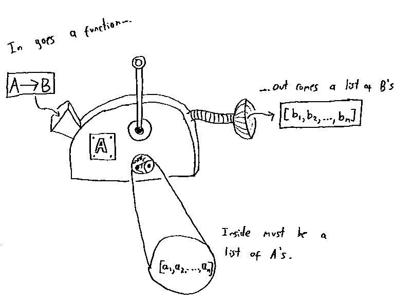
Haskell is so strict about type safety that randomly generated snippets of code that successfully typecheck are likely to do something useful, even if you've no idea what that useful thing is. This post is about what I found when I tried playing with the monad1 ListT [] even though I had no clue what purpose such a monad might serve.

I've talked about using monad transformers a couple of times. One time I looked at compositions of various types of side-effect monad, and more recently I looked at compositions of the List monad with side-effects monads. So it was inevitable that I got onto composing the List monad with itself to get ListT [].

This is literate Haskell, modulo the unicode characters.

So start with the the ordinary List monad, which is all about considering choices. For example the expression


> import Data.List
> import Control.Monad.Writer
> import Control.Monad.List

> test1 = do
> x <- [1,2,3]
> return (2*x)

> go1 = test1


can be interpreted as a program that chooses x to be each of the values 1, 2 and 3 in turn, applies f to each one and collects up the result to give [2,4,6]. The List monad will happily make choices within choices. So the expression


> test2 = do
> x <- [1,2]
> y <- [3,4]
> return (x,y)

> go2 = test2


considers, for each possible choice of x, each possible choice of y. The result is [(1,3),(1,4),(2,3),(2,4)]. More generally, for fixed sets a,b,...c the expression


do
x <- a
y <- b

z <- c
return (a,b,…,c)


returns the cartesian product a×b×…×c. In the fully general case, a,b,…c could all depend on choices that were made earlierbut right now I'm talking about the case when a,b,…,c are all 'constant'.

Here's a slightly different way of looking at this. Suppose a person called Player (P for short) is playing a solitaire game. At the first turn, P chooses a move from the set of possible first moves, then chooses a possible move from the set of second moves and so on. We can see that if we write the code

do
move1 <- possible_moves_1
move2 <- possible_moves_2

last_move <- possible_last_moves
return (move1,move2,…,last_move)

the result is a list, each of whose elements is the sequence of possible plays in the game. If the possible_*; are all 'constant' then its just the cartesian product of the plays at each turn. But it's straightforward to adapt this code to enumerate all possible plays in a more general solitaire game - and that's exactly how the List monad is sometimes used to solve such games.

So if List is about making choices, composing List with itself might seem to be about making two types of choice. And the most familiar situation where you need to iterate over two possible types of choices comes when you consider two player games. So I'll tell you a possible answer now: ListT [] is the game analysis monad!

Let's look at some examples of code in the ListT [] monad. As I pointed out earlier, we use lift a when we want a to be a list in the inner monad and mlist a when we want a to be a list in the outer monad. So in ListT [] we can expect to use both of these with lists. Consider


> mlist :: MonadPlus m => [a] -> m a
> mlist = msum . map return

> test3 = do
> a <- lift [1,2]
> b <- mlist [3,4]
> return (a,b)

> go3 = runListT test3


The value is [[(1,3),(1,4)],[(2,3),(2,4)]]. There's a nice interpretation of this. Introduce a new player called Strategist (S for short). Think of lift as meaning a choice for S and mlist as a choice for P. We can read the above as: for each first play a that S could make, go through all the first plays b that P could make. What's different from the solitaire example is how the plays have been grouped in the resulting list. For each decision S could have made, all of P's possible plays have been listed together in a sublist. But now consider this expression:


> test4 = do
> b <- mlist [3,4]
> a <- lift [1,2]
> return (b,a)

> go4 = runListT test4


We get: [[(3,1),(4,1)],[(3,1),(4,2)],[(3,2),(4,1)],[(3,2),(4,2)]]. Maybe you expect to see the same result as before but reordered. Instead we have a longer list. Our interpretation above no longer seems to hold. But actually, we can salvage it?

Go back to thinking about solitaire games. We can read the code for test2 as follows: First choose a value for x, ie. x=1. Now choose a value for y, ie. y=3. Put (1,3) in the list. Now backtrack to the last point of decision and choose again, this time y=4. Put (1,4) in the list. Now backtrack again. There are no more options for y so we backtrack all the way back to a again and set x=1, and now start again with y=3, and so on.

Now we can reconsider test4 in a two player game. Think about the choices from the point of view of working through all of P's options while fixing one particular set of choices for S. (It took me a while to get this concept so I'll try to explain this a few different ways.) So P chooses b=3 and then S makes some choice, say a=1. Now we backtrack to P's next option, b=4. But on backtracking to P's last choice we backtracked through S's choice and on running forward again, we must make some choice for S, say a=1 again. There were 2 ways P could have played, so we end up with two distinct sequences of plays: (3,1) and (4,1) after P has worked through all of his options. We have a list with two possibilities: [(3,1),(4,1)]. But S could have played differently. In fact, because we play S's move twice for each sequence of P's moves there are three other ways this sequence could have come out, depending on S's strategy: [(3,1),(4,2)], [(3,2),(4,1)] or [(3,2),(4,2)]. And that is exactly what test4 gave: for each strategy that S could have chosen we get a list of all the ways P could have played against it. We get a list of 4 lists, each of which has two elements. Each of those elements is a sequence of plays.

I'll try to make precise what I mean by 'strategy'. By strategy we mean a way of choosing a move as a function of the moves your opponent has made. That's what we mean by a program t play a game: we give it a set of inputs and it then responds with a move. Its move at the nth turn is a function of everything you did for the previous n-1 turns. So consider the example above. After P has chosen from [3,4], S must choose from [1,2]. So S's strategy can de described by a function from [3,4] to [1,2]. There are 4 such functions. Once we've fixed S's strategy, there are 2 possible ways S can play against it. Again, we have 4 strategies, and 2 plays for each strategy.

And here's another way of looking at this. We'll go back to simple games where the set of options available at each stage are constant and independent of the history of the game. Let <A,B> mean a game where A is the set of S's strategies and B is the set of ways P can play against those strategies. (The set B doesn't depend on S's choice from A because we're now limited to 'simple' games.) Now introduce a binary operator * such that <A,B>*<C,D> is the game where the moves start off being those in <A,B> but when that's finished we move onto <C,D>. In <A,B>*<C,D>, P's options are simply B×D. So we know that in some sense <A,B>*<C,D>=<X,B×D> for some X. Now S's first move is from A so that bit's easy. S's second move from C depends on P's move from B. So S's second move is described by a function from B to C. So <A,B>*<C,D>≅<A×CB,D>. (I use ≅ because I mean 'up to isomorphism'. CB×A also describes S's strategies equally well.) * is a curious binary operation. It might not look it, but it's associative (up to ismorphism). And it has a curious similarity to the semidirect product of groups. Anyway, we can write test4 using this notation. It's computing <[1],[3,4]>*<[1,2],[1]> (up to isomorphism). [1] is just a convenient way of saying "no choice" and it gives us a way to allow P to move first my making S's first move a dummy one. Multiplying gives <[1,2][3,4],[3,4]>. [1,2][3,4] has 4 elements. So again we have 4 strategies with two ways to play against each of those strategies.

It's interesting to look at <A,B>*<C,D>*<E,F>. This is <A×CB,B×D>*<E,F> which is <A×CB×EB×D,B×D×F>. This has a straightforward explanation: S gets to choose from A directly, to choose from C depending on how P plays from B and to choose from E depending on how P plays from both B and D.

And yet another way of looking at things. Suppose S and P are going to play in a chess tournament with S playing first. Unfortunately, before setting out on the journey to the tournament S realises he’s going to be late and is going to be unable to communicate during the journey. What should S do? A smart move would be to email his first move to the tournament organisers before leaving on the journey. That would buy him time while P thinks of a response. Even better, S could additionally send a list of second moves, one for each move that P might take in his absence. Going further, S could send a list of third moves, one for each of the first two moves that P might take in his absence. These emails, containing these lists, are what I’m calling a strategy. When you enumerate a bunch of options in the ListT [] monad you end up enumerating over all strategies for S and all responses for P.

It appears there’s a kind of asymmetry. Why are we considering strategies for S, but plays for P? This is partly explained by the above paragraph. In ListT [] there is an implicit ordering where S’s moves are considered to be before P’s. So if one of S’s choices comes after P’s, it needs to be pulled before P’s and that can only happen if it’s replaced with a strategy. There’s also another interesting aspect to this. When considering how to win at a game, you don’t need to test your strategy against every possible strategy your opponent might have. You only need to test it against every possible way your opponent could play against it and they only need to find one play to show your strategy isn’t foolproof. So ListT [] describes exactly what you need to figure out a winning strategy for a game.

Anyway, that’s enough theory. Here an application. The following code computes a winning strategy in the game of Nim. (If you don’t know Nim, then you’re in for a treat if you read up on it here. The theory is quite beautiful, but I deliberately don't use it here.) It uses brute force to find a winning strategy for S and additionally outputs a proof that this is a winning strategy by listing all possible ways the game could play out. Note that I’m using the WriterT String (ListT []) monad so I can log the moves made in each game.

I've also added another game, a variant of Kayles that I call Kayles'. In Kayles' there are n skittles in a row. On your turn you knock over a skittle and whichever of its immediate neighbours are still standing. The winner is the person who knocks over the last skittle. (The code describes the rules better than English text and you can adapt the code easily to play on any graph.)

Evaluate nim or kayles' to get a display of a winning strategy and a proof that it wins ie. a list of all possible games against that strategy showing they lead to P losing.


> strategies moves start = do
> a <- lift $ lift $ moves start
> tell $ [a]
> let replies = moves a
> if replies==[] then return () else do
> b <- lift $ mlist $ replies
> tell $ [b]
> strategies moves b

> nim = mapM print $
> runListT $ execWriterT $ strategies moves start
> where
> start = [2,3,5]
> moves [] = []
> moves (a:as) = [a':as | a' <- [0..a-1]]
> ++ [a:as' | as' <- moves as]

> kayles' = print $ head $
> runListT $ execWriterT $ strategies (kmoves (nbhd verts)) verts
> where
> kmoves nbhd v = [v \\ nbhd i | i <- v]
> verts = [1..13]
> nbhd verts i = intersect verts [i-1,i,i+1]


For example nim starts [[[2,3,1],…]] because a move to piles of size 2, 3 and 1 is a win in Nim. (2⊕3⊕1=0 for those who know the theory.) kayles' starts [[[1,2,3,4,5,9,10,11,12,13],…]] which means a winning move is to knock down skittles 6, 7 and 8 (you may see why symmetry makes this an obvious good opening move).

DISCLAIMER: I'm not claiming this is a good algorithm for solving games. Just that it illustrates the meaning of ListT [].

Finally a question. Are all monad transformers a form of semidirect product?

Footnotes:

[1] I haven't worked out the details but ListT [] probably isn't actually a monad. But it's close enough. It's probably associative up to ordering of the list, and as I'm using List as a poor man's Set monad2, I don't care about ordering. An alternative ListT is provided here. I'm not sure that solves the problem.


[2] I'm pretty sure Set can't be implemented in Haskell as a monad. But that's another story.

Wednesday, October 04, 2006

Negative Databases

Protecting Data Privacy through Hard-to-Reverse Negative Databases is an entertaining paper. Here's the problem it tries to solve: You want to store personal details but you don't want people to be able to mine the database. For example you might want to store brief personal details with a social security number so you can verify that someone is a member of some organisation, but for security reasons you don't want a hacker to be able to get a list of members even if they steal the entire database. That sounds like an impossible set of requirements. But the trick is this: instead of storing the personal details you store a list of all possible bitstrings representing personal details that members don't have. Insane right?


If the personal details are just 256 bits long, say, then to store details for 100 people, say, the database needs 2256-100 entries. That's vast. But the database of non-members is highly compressible. Let me lift an example directly from the papers. Suppose the personal information is three bits long and we wish to store the entries {000,100,101}. Then the non-entries are {001,010,011,110,111}. The non-entries can now be compressed using a wildcard scheme {001,*1*}. The *1* represents all of the entries fitting that pattern from 010 to 111. This turns out to be quite a compact representation. It's beginning to look plausible.


And here's the neat bit: SAT can be translated into the problem of finding valid database entries from the wildcard representation. So extracting entries is provably NP-complete, despite the fact that we can check entries in a reasonable amount of time (for suitable definitions of 'reasonable').


Anyway, I still have a whole slew of objections, and the actual compression scheme proposed has holes in it that can result in false positives. But what initially sounded implausible is beginning to look workable.


PS You can also read about this at the Economist but I've tried to spare you the irrelevant fluff :-)

Friday, September 29, 2006

Infinitesimal Types

<mad thought>I want to combine two things I've previously discussed: Synthetic Differential Geometry (SDG) and Derivatives of Containers.


SDG is all about working with values, d, such that d²=0. When this is true, we find that for suitable functions f,


f(x+d)=f(x)+d f'(x)      (Eq. 1)

where f' is the derivative of f.


Now consider derivatives of types. I've written a really sloppy description here but for a proper treatment there are papers like this one. The curious idea is that if you 'differentiate' the type of a container you find the type of the container with a hole in it. Here's a really quick example: let F[X] be the container that is a triples of X's. In other words F[X]=X×X×X=XXX=X3. Here × is the usual product in the category of types. By a container with a 'hole' we mean a container with one of its elements missing, but with a 'hole' left behind so we know where the element has gone missing from. Consider the triple. Either the first element is missing. In this case there are two elements left, so we have something of type X2. On the other hand the middle element could be missing, and the remaining elements also give something of type X2. Or the last element could be missing. Put these three cases together and we get X2+X2+X2=3X2. (The '3' in 3X² indicates that we know which of the three elements has been replaced with a hole.) If we use the prime symbol to mean differentiation we see that a triple with a hole in it is just dX3/dX=F'[X]. This generalises to other types, you can read the papers for more details. I think that's the most amazing bit of computer science I've seen in years. And it's even more fun with recursive types because you then get zippers.


Anyway, those are my ingredients and the following assumes that the above makes some kind of sense to you. So the mad thought I had was this: if you can do calculus by introducing infinitesimals such that d2=0, can we investigate containers with holes by introducing some kind of infinitesimal type with the bizarre property that

D2=0?

D is a type here, not a value. I'm hoping you can just play along here. Clearly we're talking about a weird kind of product when the product of a non-trivial object with itself is the zero object. Presumably to make sense of this we're not really talking about the usual categorical product, just as in the algebra R[d]/(d2) we're not talking about the usual real number multiplication. And note, of course, that I'm not saying that D is the type of infinitesimal numbers - I'm saying that the type itself is in some sense infinitesimal.


So what could D2=0 possibly mean? Well 0 is the type defined by the property that there are no values of type 0. So D2=0 simply means that you can't have a pair of objects of type D. So D isn't so weird at all, it corresponds to a type representing the singleton pattern. (Don't confuse this with the 'singleton' type 1. There is only one object of type 1 but we can have as many of them as we like. On the other hand, there may be many values an object of type D could take, but only one of those possible values can be realised.)


So now consider the type F[X+D]. This is a container, each of whose elements are of type X or of type D. Consider the case that they're all of type X. Then we have something of type F[X]. Now suppose that one of the elements is of type D. Then what we have is an F-container of X's with a hole, with a D in the hole. In other words, D×F'[X]. And now's the fun bit - this is all of the possible cases because the container can only contain one D. After all only one D can exist. Writing this out formally we get:

F[X+D]=F[X]+D F'[X]

In other words, we have interpreted Equation 1 in the context of types. As d can be thought of an infinitesimal value it makes sense to call D an infinitesimal type. I'm not sure how far you can run with this idea, but given that the argument above seems to make some kind of sense I expect a smarter person than me could give it rigorous form.


A final thought: D2=0 isn't really all that weird. We're already familiar with linear types and linear logic where we have things that can't be duplicated. This is just a different language to say something similar. Anyway, </mad thought>

Sunday, September 24, 2006

You can fire me, but you can't stop me working!

In my last post I had a diagram consisting of a circle and a line tangent to it. I produced this using Grapher.app which comes with MacOS X, though unless you have a good look in /Applications/Utilities you might not realise it exists. This is the latest incarnation of Apple's graphing calculator. All I had to do was plot the graphs of y=0 and x2+(y-1)2. And while it's a neat little application, what's really cool about it is the story of how it came into existence. It's an old story now, but lots of people still seem not to have heard it. It was developed illicitly, on Apple property, using Apple equipment, by an unpaid ex-Apple contractor who simply refused to leave. And despite the fact that he had to dodge his way around building security, and his project didn't show up on any official documentation, he managed to get resources allocated to his project and ultimately sneak his app onto the master disk image containing the release build of MacOS for the Power PC!


You can either read the full version of the story here or, and this is the version I recommend, you can listen to the programme from This American Life.

Update: Ron Avitzur contacted me to point out that Grapher is a separate application to Graphing Calculator. But I presume that Apple intended Grapher to be a followup to Graphing Calculator. Graphing Calculator is still being developed and I'll be playing with both apps now.

Thursday, September 21, 2006

Practical Synthetic Differential Geometry

Previously I've talked about Automatic Differentiation (AD). My own formulation of the technique is more algebraic than the description that is usually given, and recently it's begun to dawn on me that all I've done is rediscover Synthetic Differential Geometry (SDG). I've looked at a variety of SDG papers but none of them seem to make the connection with AD. This is a pity because SDG allows you to do an amazing thing - write computer programs that easily manipulate objects such as vector fields and differential forms on manifolds without doing symbolic algebra. My goal here is to illustrate how the definition of vector field in Anders Kock's book gives a nice functional definition of a vector field and how that definition leads naturally to the Lie bracket. Normally it takes a significant amount of mathematical machinery to define these things but in the framework of SDG it becomes very simple. (Unfortunately this is going to be very sketchy as there's a lot I could say and I only have a small amount of time while I sit at home waiting for a new TV to be delivered...)

Kock's work is based on the idea of infinitesimal numbers whose square is zero but which aren't themselves zero. Clearly we aren't talking about real numbers here, but instead an extension to the real numbers. Here's a toy implementation:


> data Dual a = D a a deriving (Show,Eq)

> instance Num a => Num (Dual a) where
> fromInteger i = D (fromInteger i) 0
> (D a a')+(D b b') = D (a+b) (a'+b')
> (D a a')-(D b b') = D (a-b) (a'-b')
> (D a a')*(D b b') = D (a*b) (a*b'+a'*b)

> e = D 0 1


They're called dual numbers because this particular algebra was apparently first described by Clifford and that's what he called them. The important point to note is that e^2==0. We can use the fact that
f(x+e)=f(x)+ef'(x)

to compute derivatives of functions. For example if we define


> f x = x^3+2*x^2-3*x+1


and evaluate f (1+e) we get D 1 4. We can directly read off f(1)=1 and f'(1)=4.

But, as Kock points out, the dual numbers don't provide 'enough' infinitesimals, we just get one, e, from which all of the others are built. So we can replace Dual with a new class:


> infixl 5 .-
> infixl 5 .+
> infixl 6 .*
> infixl 6 *.

> data R a = R a [a] deriving Show

> zipWith' f l r [] [] = []
> zipWith' f _ r a [] = map (flip f r) a
> zipWith' f l _ [] b = map (f l) b
> zipWith' f l r (a:as) (b:bs) = (f a b) : zipWith' f l r as bs

> (.+) :: Num a => [a] -> [a] -> [a]
> (.+) = zipWith' (+) 0 0

> (.-) :: Num a => [a] -> [a] -> [a]
> (.-) = zipWith' (-) 0 0

> (.*) :: Num a => a -> [a] -> [a]
> (.*) a = map (a*)

> (*.) :: Num a => [a] -> a -> [a]
> (*.) a b = map (*b) a

> (.=) :: (Eq a,Num a) => [a] -> [a] -> Bool
> (.=) a b = and $ zipWith' (==) 0 0 a b

> instance (Eq a,Num a) => Eq (R a) where
> R a a' == R b b' = a==b && a'.=b'


A slightly more extended version of the Num interface:


> instance Num a => Num (R a) where
> fromInteger a = R (fromInteger a) []
> (R a a') + (R b b') = R (a+b) (a'.+b')
> (R a a') - (R b b') = R (a-b) (a'.-b')
> (R a a') * (R b b') = R (a*b) (a.*b' .+ a'*.b)
> negate (R a a') = R (negate a) (map negate a')


And some more functions for good measure:


> instance (Num a,Fractional a) => Fractional (R a) where
> fromRational a = R (fromRational a) []
> (R a a') / (R b b') = let s = 1/b in
> R (a*s) ((a'*.b.-a.*b') *. (s*s))

> instance Floating a => Floating (R a) where
> exp (R a a') = let e = exp a in R e (e .* a')
> log (R a a') = R (log a) ((1/a) .* a')
> sin (R a a') = R (sin a) (cos a .* a')
> cos (R a a') = R (cos a) (-sin a .* a')


The d i provide a basis for these infinitesimals.


> d n = R 0 (replicate n 0 ++ [1])


We now have an infinite set of independent dual numbers, d i, one for each natural i. Note that we have (d i)*(d j)==0 for any i and j. Apart from this, they act just like before. For example
f(x+di)=f(x)+dif'(x).

We can use these compute partial derivatives. For example consider


> g x y = (x+2*y)^2/(x+y)


Computing g (7+d 0) (0+d 1) gives R 7.0 [1.0,3.0] so we know g(7,0) = 7, gx(7,0)=1 and gy(7,0)=3.

I'll use R as mathematical notation for the type given by R Float. (I hope the double use of 'R' won't be confusing, but I want to be consistent-ish with Kock.)

Before we do any more calculus, consider the following geometric figure:


A point is in the intersection of the circle and the line if it satisfies the equations:


> onS (x,y) = x^2+(y-1)^2==1
> onL (x,y) = y==0


Notice that in R this has many solutions. In fact, we find that onS (a*d 1,0) && onL (a*d 1,0) gives True for any Float value a. Does this mean anything? Actually, it fits some people's intuition of what the intersection should look like better than the usual idea that there is only one intersection point. In fact, Protagoras argued that there was a short line segment in common between the circle and the line and that because Pythogoras's theorem gave only one solution the whole of geometry was at fault! Using R instead of the reals makes sense of this intuition. The points of the form (a*d 1,0) do, indeed, form a line tangent to the circle. In fact, there is a way to construct tangent spaces and vector fields directly from this - but instead I want to now consider Kock's construction which is slightly different.

Let D be the subset of R consisting of numbers whose square is zero. These numbers are in some sense infinitesimal. In differential geometry a vector field is intuitively thought of as an 'infinitesimal flow' on a manifold. A finite flow on a manifold, M, is simply a function f:R×M→M such that f(x,0)=0. In f(x,t) we can think of t as time and each point x on the manifold flows along a path t→f(x,t). If f is differentiable, then as t becomes smaller, the path becomes closer and closer to a short line segment which we can draw as a vector. So the intuition is that a vector field is what you get in the limit as t becomes infinitesimal. The catch is that infinitesimal things aren't first class objects in differential geometry (so to speak). You can use infinitesimals for intuition, and I suspect almost all differential geoneters do, but actually talking about them is taboo. In fact, the definition of vector field in differential geometry is a bit of a kludge to work around this issue. When most people first meet the definition of a vector field as a differential operator it comes as quite a shock. But we have no such problem. In fact, Kock defines a vector field simply as a function
f:D×M→M
such that f(0,x)=x.
In the language of SDG, a vector field is an infinitesimal flow. For example, consider


> transX d (x,y) = (x+d,y)


This simply translates along the x-axis infinitesimally. Of course this code defines a flow for non-infinitesimal values of d, but when considering this as a vector field we're only interested in when d is infinitesimal. transX defines a vector field that everywhere points along the x-axis.

For those familiar with the usual differential geometric definition of vector fields I can now make contact with that. In that context a vector field is a differential operator that acts on scalar functions on your manifold. In our case, we can think of it acting by infinitesimally dragging the manifold and then looking at what happens to the function that's dragged along. In other words, if we have a funtion, f, on the manifold, the vector field v, applied to f, is that function vf such that f (f d x)==f x + d*vf x. For example with


> h (x,y) = x^2+y^2


h (transX (d 1) (1,2)) == R 5 [2] because h(x,y)=5 and hx(x,y)=2.

I think I have enough time to briefly show how to define the Lie bracket in this context. If you have two vector fields, then intuitively you can view the Lie bracket as follows: take a point, map it using the first field by some small parameter d1, then map it using the second for time d2, then doing the first one by parameter -d1, and then the second by -d2. Typically you do not return to where you started from, but somewhere 'close'. In fact, your displacement is proportional to the product of d1 and d2. In other words, if your fields are v and w, then the Lie bracket [v,w] is defined by the equation v (-d2) $ v (-d1) $ w d2 $v d1 x==vw (d1*d2) x where vw represents [v,w]. But you might now see a problem. The way we have defined things d1*d2 is zero if d1 and d2 are infinitesimal. Kock discusses this issue and points out that in order to compute Lie brackets we need infinitesimals whose squares are zero, but whose product isn't. I could go back and hack the original definition of R to represent a new kind of algebraic structure where this is true, but in the spirit of Geometric Algebra for Free I have a trick. Consider d1=1⊗d and d2=d⊗1 in R⊗R. Clearly d12=d22=0. We also have d1d2=d⊗d≠0. And using the constructor as tensor product trick we can write:


> d1 = R (d 0) [] :: R (R Double)
> d2 = R 0 [1] :: R (R Double)


Let's test it out. Define three infinitesimal rotations:


> rotX d (x,y,z) = (x,y+d*z,z-d*y)
> rotY d (x,y,z) = (x-d*z,y,z+d*x)
> rotZ d (x,y,z) = (x+d*y,y-d*x,z)


Note that there's no need to use trig functions here. We're working with infinitesimal rotations so we can use the fact that sin d=d and cos d=1 for infinitesimal d. It is well known that [rotX,rotY]=rotZ and cyclic permutations thereof. (In fact, these are just the commutation relations for angular momentum in quantum mechanics.)

We can write


> commutator d1 d2 f g = (g (-d2) . f (-d1) . g d2 . f d1)

> test1 = commutator d1 d2 rotX rotY
> test2 = rotZ (d1*d2)


and compare values of test1 and test2 at a variety of points to see if they are equal. For example test1 (1,2,3) == test2(1,2,3). I don't know about you, but I'm completely amazed by this. We can get our hands right on things like Lie brackets with the minimum of fuss. This has many applications. An obvious one is in robot dynamics simulations where we frequently need to work with the Lie algebra of the group of rigid motions. This approach won't give us new algorithms, but it gives a very elegant way to express existing algorithms. It's also, apprently, close to Sophus Lie's original description of the Lie bracket.

I have time for one last thing. So far the only manifolds I've considered are those of the form Rn. But this stuff works perfectly well for varieties. For example, the rotations rotX, rotY and rotZ all work fine on the unit sphere. In fact, if T is the unit sphere define


> onT (x,y,z) = x^2+y^2+z^2==1


Notice how, for example, onT (rotY (d 1) (0.6,0.8,0))==True, so rotY really does give an infinitesimal flow from the unit sphere to the unit sphere, and hence a vector field on the sphere. Compare this to the complexity of the traditional definition of a vector field on a manifold.

Kock's book also describes a really beautiful definition of the differential forms in terms of infinitesimal simplices, but I've no time for that now. And I've also no time to mention the connections with intuitionistic logic and category theory making up much of his book (which is a good thing because I don't understand them).

PS The D⊗D trick, implemented in C++, is essentially what I did in my paper on photogrammetry. But there I wasn't thinking geometrically.

(I don't think I've done a very good job of writing this up. Partly I feel horribly constricted by having to paste back and forth between two text editors to get this stuff in a form suitable for blogger.com as well as periodically having to do some extra munging to make sure it is still legal literate Haskell. And diagrams - what a nightmare! So I hit the point where I couldn't face improving the text any more without climbing up the walls. What is the best solution to writing literate Haskell, with embedded equations, for a blog?)

Blog Archive