Practical Synthetic Differential Geometry

Previously I've talked about Automatic Differentiation (AD). My own formulation of the technique is more algebraic than the description that is usually given, and recently it's begun to dawn on me that all I've done is rediscover Synthetic Differential Geometry (SDG). I've looked at a variety of SDG papers but none of them seem to make the connection with AD. This is a pity because SDG allows you to do an amazing thing - write computer programs that easily manipulate objects such as vector fields and differential forms on manifolds without doing symbolic algebra. My goal here is to illustrate how the definition of vector field in Anders Kock's book gives a nice functional definition of a vector field and how that definition leads naturally to the Lie bracket. Normally it takes a significant amount of mathematical machinery to define these things but in the framework of SDG it becomes very simple. (Unfortunately this is going to be very sketchy as there's a lot I could say and I only have a small amount of time while I sit at home waiting for a new TV to be delivered...)

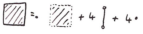
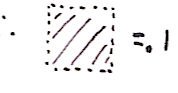
Kock's work is based on the idea of infinitesimal numbers whose square is zero but which aren't themselves zero. Clearly we aren't talking about real numbers here, but instead an extension to the real numbers. Here's a toy implementation:

> data Dual a = D a a deriving (Show,Eq)

> instance Num a => Num (Dual a) where
>   fromInteger i = D (fromInteger i) 0
>   (D a a')+(D b b') = D (a+b) (a'+b')
>   (D a a')-(D b b') = D (a-b) (a'-b')
>   (D a a')*(D b b') = D (a*b) (a*b'+a'*b) 

> e = D 0 1

They're called dual numbers because this particular algebra was apparently first described by Clifford and that's what he called them. The important point to note is that e^2==0. We can use the fact that

f(x+e)=f(x)+ef'(x)

to compute derivatives of functions. For example if we define

> f x = x^3+2*x^2-3*x+1

and evaluate f (1+e) we get D 1 4. We can directly read off f(1)=1 and f'(1)=4.

But, as Kock points out, the dual numbers don't provide 'enough' infinitesimals, we just get one, e, from which all of the others are built. So we can replace Dual with a new class:

> infixl 5 .-
> infixl 5 .+
> infixl 6 .*
> infixl 6 *.

> data R a = R a [a] deriving Show

> zipWith' f l r [] [] = []
> zipWith' f _ r a [] = map (flip f r) a
> zipWith' f l _ [] b = map (f l) b
> zipWith' f l r (a:as) (b:bs) = (f a b) : zipWith' f l r as bs

> (.+) :: Num a => [a] -> [a] -> [a]
> (.+) = zipWith' (+) 0 0

> (.-) :: Num a => [a] -> [a] -> [a]
> (.-) = zipWith' (-) 0 0

> (.*) :: Num a => a -> [a] -> [a]
> (.*) a = map (a*)

> (*.) :: Num a => [a] -> a -> [a]
> (*.) a b = map (*b) a

> (.=) :: (Eq a,Num a) => [a] -> [a] -> Bool
> (.=) a b = and $ zipWith' (==) 0 0 a b

> instance (Eq a,Num a) => Eq (R a) where
>    R a a' == R b b' = a==b && a'.=b'

A slightly more extended version of the Num interface:

> instance Num a => Num (R a) where
>    fromInteger a = R (fromInteger a) []
>    (R a a') + (R b b') = R (a+b) (a'.+b')
>    (R a a') - (R b b') = R (a-b) (a'.-b')
>    (R a a') * (R b b') = R (a*b) (a.*b' .+ a'*.b)
>    negate (R a a') = R (negate a) (map negate a')

And some more functions for good measure:

> instance (Num a,Fractional a) => Fractional (R a) where
>    fromRational a = R (fromRational a) []
>    (R a a') / (R b b') = let s = 1/b in
>        R (a*s) ((a'*.b.-a.*b') *. (s*s))

> instance Floating a => Floating (R a) where
>    exp (R a a') = let e = exp a in R e (e .* a')
>    log (R a a') = R (log a) ((1/a) .* a')
>    sin (R a a') = R (sin a) (cos a .* a')
>    cos (R a a') = R (cos a) (-sin a .* a')

The d i provide a basis for these infinitesimals.

> d n = R 0 (replicate n 0 ++ [1])

We now have an infinite set of independent dual numbers, d i, one for each natural i. Note that we have (d i)*(d j)==0 for any i and j. Apart from this, they act just like before. For example

f(x+d_i)=f(x)+d_if'(x).

We can use these compute partial derivatives. For example consider

> g x y = (x+2*y)^2/(x+y)

Computing g (7+d 0) (0+d 1) gives R 7.0 [1.0,3.0] so we know g(7,0) = 7, g_x(7,0)=1 and g_y(7,0)=3.

I'll use R as mathematical notation for the type given by R Float. (I hope the double use of 'R' won't be confusing, but I want to be consistent-ish with Kock.)

Before we do any more calculus, consider the following geometric figure:



A point is in the intersection of the circle and the line if it satisfies the equations:

> onS (x,y) = x^2+(y-1)^2==1
> onL (x,y) = y==0

Notice that in R this has many solutions. In fact, we find that onS (a*d 1,0) && onL (a*d 1,0) gives True for any Float value a. Does this mean anything? Actually, it fits some people's intuition of what the intersection should look like better than the usual idea that there is only one intersection point. In fact, Protagoras argued that there was a short line segment in common between the circle and the line and that because Pythogoras's theorem gave only one solution the whole of geometry was at fault! Using R instead of the reals makes sense of this intuition. The points of the form (a*d 1,0) do, indeed, form a line tangent to the circle. In fact, there is a way to construct tangent spaces and vector fields directly from this - but instead I want to now consider Kock's construction which is slightly different.

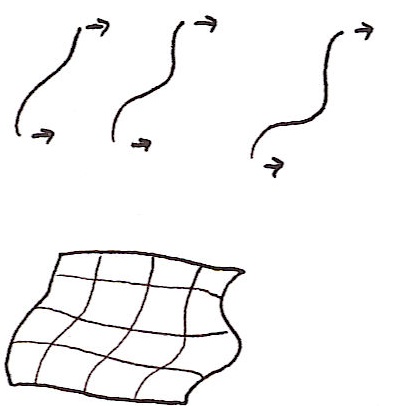
Let D be the subset of R consisting of numbers whose square is zero. These numbers are in some sense infinitesimal. In differential geometry a vector field is intuitively thought of as an 'infinitesimal flow' on a manifold. A finite flow on a manifold, M, is simply a function f:R×M→M such that f(x,0)=0. In f(x,t) we can think of t as time and each point x on the manifold flows along a path t→f(x,t). If f is differentiable, then as t becomes smaller, the path becomes closer and closer to a short line segment which we can draw as a vector. So the intuition is that a vector field is what you get in the limit as t becomes infinitesimal. The catch is that infinitesimal things aren't first class objects in differential geometry (so to speak). You can use infinitesimals for intuition, and I suspect almost all differential geoneters do, but actually talking about them is taboo. In fact, the definition of vector field in differential geometry is a bit of a kludge to work around this issue. When most people first meet the definition of a vector field as a differential operator it comes as quite a shock. But we have no such problem. In fact, Kock defines a vector field simply as a function

f:D×M→M

such that f(0,x)=x.
In the language of SDG, a vector field is an infinitesimal flow. For example, consider

> transX d (x,y) = (x+d,y)

This simply translates along the x-axis infinitesimally. Of course this code defines a flow for non-infinitesimal values of d, but when considering this as a vector field we're only interested in when d is infinitesimal. transX defines a vector field that everywhere points along the x-axis.

For those familiar with the usual differential geometric definition of vector fields I can now make contact with that. In that context a vector field is a differential operator that acts on scalar functions on your manifold. In our case, we can think of it acting by infinitesimally dragging the manifold and then looking at what happens to the function that's dragged along. In other words, if we have a funtion, f, on the manifold, the vector field v, applied to f, is that function vf such that f (f d x)==f x + d*vf x. For example with

> h (x,y) = x^2+y^2

h (transX (d 1) (1,2)) == R 5 [2] because h(x,y)=5 and h_x(x,y)=2.

I think I have enough time to briefly show how to define the Lie bracket in this context. If you have two vector fields, then intuitively you can view the Lie bracket as follows: take a point, map it using the first field by some small parameter d1, then map it using the second for time d2, then doing the first one by parameter -d1, and then the second by -d2. Typically you do not return to where you started from, but somewhere 'close'. In fact, your displacement is proportional to the product of d1 and d2. In other words, if your fields are v and w, then the Lie bracket [v,w] is defined by the equation v (-d2) $ v (-d1) $ w d2 $v d1 x==vw (d1*d2) x where vw represents [v,w]. But you might now see a problem. The way we have defined things d1*d2 is zero if d1 and d2 are infinitesimal. Kock discusses this issue and points out that in order to compute Lie brackets we need infinitesimals whose squares are zero, but whose product isn't. I could go back and hack the original definition of R to represent a new kind of algebraic structure where this is true, but in the spirit of Geometric Algebra for Free I have a trick. Consider d₁=1⊗d and d₂=d⊗1 in R⊗R. Clearly d₁²=d₂²=0. We also have d₁d₂=d⊗d≠0. And using the constructor as tensor product trick we can write:

> d1 = R (d 0) [] :: R (R Double)
> d2 = R 0 [1] :: R (R Double)

Let's test it out. Define three infinitesimal rotations:

> rotX d (x,y,z) = (x,y+d*z,z-d*y)
> rotY d (x,y,z) = (x-d*z,y,z+d*x)
> rotZ d (x,y,z) = (x+d*y,y-d*x,z)

Note that there's no need to use trig functions here. We're working with infinitesimal rotations so we can use the fact that sin d=d and cos d=1 for infinitesimal d. It is well known that [rotX,rotY]=rotZ and cyclic permutations thereof. (In fact, these are just the commutation relations for angular momentum in quantum mechanics.)

We can write

> commutator d1 d2 f g = (g (-d2) . f (-d1) . g d2 . f d1)

> test1 = commutator d1 d2 rotX rotY
> test2 = rotZ (d1*d2)

and compare values of test1 and test2 at a variety of points to see if they are equal. For example test1 (1,2,3) == test2(1,2,3). I don't know about you, but I'm completely amazed by this. We can get our hands right on things like Lie brackets with the minimum of fuss. This has many applications. An obvious one is in robot dynamics simulations where we frequently need to work with the Lie algebra of the group of rigid motions. This approach won't give us new algorithms, but it gives a very elegant way to express existing algorithms. It's also, apprently, close to Sophus Lie's original description of the Lie bracket.

I have time for one last thing. So far the only manifolds I've considered are those of the form Rⁿ. But this stuff works perfectly well for varieties. For example, the rotations rotX, rotY and rotZ all work fine on the unit sphere. In fact, if T is the unit sphere define

> onT (x,y,z) = x^2+y^2+z^2==1

Notice how, for example, onT (rotY (d 1) (0.6,0.8,0))==True, so rotY really does give an infinitesimal flow from the unit sphere to the unit sphere, and hence a vector field on the sphere. Compare this to the complexity of the traditional definition of a vector field on a manifold.

Kock's book also describes a really beautiful definition of the differential forms in terms of infinitesimal simplices, but I've no time for that now. And I've also no time to mention the connections with intuitionistic logic and category theory making up much of his book (which is a good thing because I don't understand them).

PS The D⊗D trick, implemented in C++, is essentially what I did in my paper on photogrammetry. But there I wasn't thinking geometrically.

(I don't think I've done a very good job of writing this up. Partly I feel horribly constricted by having to paste back and forth between two text editors to get this stuff in a form suitable for blogger.com as well as periodically having to do some extra munging to make sure it is still legal literate Haskell. And diagrams - what a nightmare! So I hit the point where I couldn't face improving the text any more without climbing up the walls. What is the best solution to writing literate Haskell, with embedded equations, for a blog?)

Local and global side effects with monad transformers

There is an annual puzzle event that 90 or so people attend. Each designs a puzzle and manufactures 90 copies of it which are then shared with the other participants. All 90 then get to go home with 90 puzzles.

Anyway, an ex-coworker attends this event and I had a chance to play with his puzzle. It was one of those fitting blocks together types puzzles. It was ingeniously designed but it seemed pretty clear to me that it required a lot of combinatorial searching. So I decided to write a program in Haskell to solve it using the List monad to enable simple logic programming.

But my code had a slight problem. It worked through the puzzle and found solutions, but (1) it didn't log the steps it took to achieve those solutions and (2) I couldn't count how many combinations it searched to find the solutions. Both of these could be thought of as side-effects, so the obvious thing to do is use a monad to track these things. But there was a catch - I was already using a monad - the List monad. When that happens there's only one thing for it - using a monad transformer to combine monads.

There are two distinct ways to combine a monad with the List monad and I needed both.

Anyway, this is literate Haskell. I'll assume you're vaguely familiar with using the List monad for logic programming. I also assume you're familiar with MonadPlus though that's not something I've written about here. And I couldn't get this stuff to work in Hugs, so use ghc. Here's some code:

> import Control.Monad.List
> import Control.Monad.State
> import Control.Monad.Writer

I'm not going to describe the original puzzle now. Instead I'm going to look at an almost trivial logic problem so that we can concentrate on the monad transforming. The puzzle is this: find all the possible sums of pairs of integers, one chosen from the set {1,2} and the other from the set {2,4}, where the sum is less than 5. Here's a simple implementation.

> test1 :: [Integer]

> test1 = do
>     a <- [1,2]
>     b <- [2,4]
>     guard $ a+b<5
>     return $ a+b

> go1 = test1

Run go1 and you should get the result [3,4]. But that's just the sums. What were the pairs of integers that went into those sums? We could simply return (a,b,a+b), but in more complex problems we might want to log a complex sequence of choices and that would entail carrying all of that information around. What we'd like is to simply have some kind of log running as a side effect. For this we need the Writer monad.

If you cast your mind back, monad transformers layer up monads a bit like layers of onion skin. What we want is to wrap a List monad in a Writer monad. We do this using the WriterT monad transformer. All we have to do is add a tell line to our code, and use 'lift' to pull the items in the list monad out from one layer of onion. Here's what the code looks like:

> test2 :: WriterT [Char] [] Integer

> test2 = do
>     a <- lift [1,2]
>     b <- lift [2,4]
>     tell ("trying "++show a++" "++show b++"\n")
>     guard $ a+b<5
>     return $ a+b

To get the final result we need to use runWriterT to peel the onion:

> go2 = runWriterT test2

Execute go2 and we get a list of pairs of sums and logged messages.

There's an important point to note here: we have one log per sum, so the logs are 'local'. What if we want a 'global' side effect such as a count of how many combinations were tried, regardless of whether they succeded or failed? An obvious choice of monad to count attempts is the State monad, but to make its effects 'global' we now need to make State the inner monad and make List provide the outer layer of skin. We're wrapping the opposite way to in the previous example. And now there's a catch. We use a line like a <- [1,2] to exploit the List monad. But now we no longer have a List monad, instead we have a ListT (State Integer) monad. This means that [1,2] is not an object in this monad. We can't use 'lift' either because the inner monad isn't List. We need to translate our lists into the ListT (State Integer) monad.

We can do slightly better, we can translate a list from the List monad into any other instance of MonadPlus. Remember that return x :: [X] is the same as [x] and x ++ y is the same as x `mplus` y :: [X]. For example [1,2] == (return 1) `mplus` (return 2). The latter only uses functions from the MonadPlus interface to build the list, and hence it can be used to build the equivalent of a List in any MonadPlus. To mplus a whole list we use msum leading to the definition:

> mlist :: MonadPlus m => [a] -> m a
> mlist = msum . map return

As a function [a] -> [a], mlist is just the identity. Now we're ready to go:

> test3 :: ListT (State Integer) Integer

> test3 = do
>     a <- mlist [1,2]
>     b <- mlist [2,4]
>     lift $ modify (+1)
>     guard $ a+b<5
>     return $ a+b

> go3 = runState (runListT test3) 0

Run go3 to see the result. Note we had to lift the modify line because the State monad is the inner one.

And now we have one more problem to solve: bouth logging and counting simultaneously:

> test4 :: WriterT [Char] (ListT (State Integer)) Integer

> test4 = do
>     a <- lift $ mlist [1,2]
>     b <- lift $ mlist [2,4]
>     tell ("trying "++show a++" "++show b++"\n")
>     lift $ lift $ modify (+1)
>     guard $ a+b<5
>     return $ a+b

> go4 = runState (runListT $ runWriterT test4) 0

That's it!

We can carry out a cute twist on this. By swapping the innermost and outermost monads we get:

> test5 :: StateT Integer (ListT (Writer [Char])) Integer

> test5 = do
>     a <- lift $ mlist [1,2]
>     b <- lift $ mlist [2,4]
>     lift $ lift $ tell ("trying "++show a++" "++show b++"\n")
>     modify (+1)
>     guard $ a+b<5
>     return $ a+b

> go5 = runWriter $ runListT $ runStateT test5 0

go5 returns a local count of how many combinations were required for each problem, and the Writer monad now records every 'try' in one long log.

One last thing: you don't need to explicitly 'lift' things - the monad transformers have a nice interface that automatically lifts some operations. (You may need a recent Haskell distribution for this, it fails for older versions.)

> test6 :: WriterT [Char] (ListT (State Integer)) Integer

> test6 = do
>     a <- mlist [1,2]
>     b <- mlist [2,4]
>     tell ("trying "++show a++" "++show b++"\n")
>     modify (+1)
>     guard $ a+b<5
>     return $ a+b

> go6 = runState (runListT $ runWriterT test6) 0

It'd be cool to get rid of the mlist too. Maybe if the Haskell parser was hacked so that [1,2] didn't mean 1:2:[] but instead meant (return 1) `mplus` (return 2) like the way Gofer interprets list comprehensions in any monad. (For all I know, Gofer already does exactly what I'm suggesting.)

One thing I should add - these monad transformers really kill performance. The puzzle solver I wrote no longer gives me any solutions in the few minutes that it used to...

PS I just made up the mlist thing. There may be a better way of doing this that I don't know about. I was surprised it wasn't already in the Control.Monad library somewhere. mlist is kind of a homomorphism between MonadPlusses and I think it might make the List MonadPlus an initial object in some category or other - but that's just speculation right now.

Update: I fixed the non-htmlised <'s. I think it takes more time to convert to blogger-compatible html than to write my posts! Also take a look at this. My mlist corresponds to their liftList - and now I know I wasn't completely off the rails writing mlist.

More Low Cost Geometric Algebra

In my second last post I showed how large algebraic structures could be built out of smaller ones using parametric polymorphism. In fact, for certain types, the type constructor acts like a tensor product in the category of algebras. It turns out that many of these structures are isomorphic to each other and Haskell provides a nice way to talk about these isomorphisms.

Before that I should say a bit more about Clifford algebras. These are an important tool in many branches of mathematics - algebraic topology, K-theory, representation theory and in theoretical physics. But one interesting aspect is that they can provide an alternative to the usual vector language of geometry. Many people will be familiar with the use of quaternions to represent 3D rotations. Clifford algebras generalise this to N-dimensions.

Before proceeding, note the footnote below on notation. And rather than write literate Haskell I've put the code here.

Back on topic: the first isomorphisms I should mention are

A⊗B≅B⊗A

for any A and B. For example H⊗R(2)≅R(2)⊗H. As Haskell types this says that Quaternion (Matrix a) is isomorphic to Matrix (Quaternion a). Or in English: the 2×2 matrices of quaternions are isomorphic to the quaternions whose components are 2×2 matrices. This isn't completely trivial. For example let ms2sm be the isomorphism

ms2sm :: (Num a) => Matrix (Split a) -> Split (Matrix a)
ms2sm (M (S a b) (S c d) (S f g) (S h j)) =
    S (M a c f h) (M b d g j)

You can see that it's a little like a matrix transpose operation.

We can draw this pictorially as:


Note that the same function, because it is polymorphic, also gives an isomorphism Matrix (Split (Quaternion a)) -> Split (Matrix (Quaternion a)). But what about the isomorphism Quaternion (Matrix (Split a)) -> Quaternion (Split (Matrix a))? We can get this almost for free using the functoriality of the constructors. The isomorphism is fmap ms2sm. We can illustrate this as:

If we implement each of the pairwise flips then in combination with fmap we can get any permutation of the constructors. And you can probably imagine some pretty braid-like diagrams describing the process. (I could mutter something about symmetric monoidal categories here.)

These isomorphisms are almost trivial - they just swap elements around. But pick up any book that discusses Clifford algebras and you'll find a bunch of extra isomorphisms listed:

C⊗C≅C⊕C

C⊗H≅C(2)

H⊗H≅R(4)

For example, a quaternion of quaternions is much the same as a 4×4 matrix. We choose to represent the latter as a 2×2 matrix of 2×2 entries with the isomorphism

qq2mm :: (Num a) => Quaternion (Quaternion a) -> Matrix (Matrix a)
qq2mm (Q (Q a b c d) (Q f g h j) (Q k l m n) (Q p q r s)) =
    M (M (a+g+m+s) (b-f-n+r)  (f-b-n+r)  (a+g-m-s))
      (M (c+j-k-q) (d-h+l-p)  (h-d+l-p)  (c+j+k+q))
      (M (j-c+k-q) (d+h+l+p)  (-d-h+l+p) (j-c-k+q)
      (M (a-g+m-s) (-b-f+n+r) (b+f+n+r)  (a-g-m+s))

(That took me a few minutes of actual work to unpack the proof of that in Spin Geometry by Lawson and Michelson so it's no longer for free!) There's a really important reason why you might want to do this. It takes 16 multiplications of the underlying elements to multiply two quaternions but it only takes 8 multiplications to multiply 2×2 matrices. A Matrix (Matrix a) can therefore be multiplied four times as fast as a Quaternion (Quaternion a). So being able to switch back and forth between repesentations is useful.

I think I now have a simple kit of parts for manipulating Clifford algebras efficiently. If I have time I should try to write a complete library for N-dimensional Clifford algebras. I wonder if I could apply it to path counting methods?

Back to isomorphisms. I want to mention two in particular. One is

C_n+8=R(16)⊗C_n

The actual isomorphism is

bott :: Num a => Quaternion (Matrix (Quaternion (Matrix a))) -> Matrix (Matrix (Matrix (Matrix a)))
bott = qq2mm . fmap mq2qm

It's prettier viewed pictorially:


As I've mentioned before, this isomorphism is an example of Bott periodicity. It pops up in many places in mathematics, for example in Supergravity or K-Theory.

This is an interesting isomorphism:

Remember that Split a is essentially a pair of objects of type a. So we can define

cliff72left,cliff72right :: Cliff7 -> Matrix (Matrix (Matrix R))
cliff72left = first . ms2sm . fmap ms2sm . (fmap (fmap ms2sm)) . qq2mm . fmap mq2qm
cliff72right = second . ms2sm . fmap ms2sm . (fmap (fmap ms2sm)) . qq2mm . fmap mq2qm

This gives not one, but two different ways to represent an element of C₇ as an 8×8 matrix. But there's more to it than that. The main real-world application for quaternions is for describing rotations - they're well used in the 3D graphics world for example. Elements of C₇ can be used to describe rotations in 8D. (Modulo a sign ambiguity that should be familiar to anyone who's played with quaternions.) So what he have is that a rotation in 8D can be represented with 3 different 8×8 matrices: the usual one, and the two coming from C₇ (modulo the sign). This has many implications in physics. For example these three matrices describe how bosons, left-handed fermions and right-handed fermions transform under rotations. In 8-dimensions these matrices are all 8×8 making 8D a special dimension for doing physics. By a roundabout path this is closely linked to the 10D of superstring theory. This "theewayness" is known as triality which John Baez has written about a few times.

I'm getting to like this type constructor as tensor product viewpoint. I can see a lot of mathematics that be expressed nicely in it. General relativity and knot theory are two that come to mind...

Footnote about notation

I go back and forth between conventional mathematical notation and Haskell. I also have one letter abbreviations I use in function names and diagrams. The translation table is:

Mathematics	Haskell	Abbreviation
R⊕R	Split	s
C	Complex	c
H	Quaternion	q
R(2)	Matrix	m
Cn	CliffN
C'n	CliffN'

Learn Maths with Haskell

This is a quick plug for the web site of a friend of mine, David Amos. He's been working hard to produce a treasure trove of useful mathematical code in Haskell with the intention of making abstract objects more accessible to mathematics learners.

Highlights include code for

1. Commutative algebra, including Gröbner basis computation and tools for manipulating ideals of rings.
   
2. Permutation groups, including an implementation of the Schreier-Sims algorithm and tools for investigating the Rubik's cube group and its subgroups.
   
3. Number theory. Includes tools for working with quadratic fields, p-adic numbers and elliptic curves, and code for factoring using Lenstra's elliptic curve algorithm.
   

The full repository is here. (Use that link to download the code as some of the other links appear to be broken right now.)

It'd be great to see a textbook grow out of some of this work...

Geometric Algebra for Free!

I'm a fan of Haskell. But I'm not a zealot. I'll be the first to tell you that some of the stuff down below works better in C++. But C++ has syntax uglier than a mandrill's rear end so I'll sacrifice functionality for readability. This is literate Haskell by the way. Copy and paste this whole entry into a .lhs file and run it with hugs -98 or ghci -fglasgow-exts.

The first bit of functionality I'll sacrfice is some of the genericity of my code so let's start with fixing a base field. Everything I say below will be over the reals:

> type R = Float

Anyway, today's theme is about how writing your code generically allows you to combine classes together in unanticipated ways to give you useful stuff - more or less for free.

If you've done some mathematical coding you probably have a complex number class lying around somewhere. If it's written in a modern language it's probably generic allowing you to choose your base structure. For example in C++ you might be able to use complex<float> or complex<int>. If you don't have such a class you can have a Haskell one for free:

> data Complex a = C a a deriving (Eq,Show)

> instance Num a => Num (Complex a) where
>     fromInteger a = C (fromInteger a) 0
>     (C a b)+(C a' b') = C (a+a') (b+b')
>     (C a b)-(C a' b') = C (a-a') (b-b')
>     (C a b)*(C a' b') = C (a*a'-b*b') (a*b'+b*a')

The usual complex numbers are given by Complex R. But here's a question: does Complex (Complex R) mean anything. Complex a requires a to be a Num, but Complex R is a Num. So Complex (Complex R) compiles fine. But does it mean anything mathematically? It does, it corresponds to C⊗C. (Remember, I'm working over the reals, so by ⊗ I mean ⊗_R.) If you're shaky on tensor products then I can give a one line summary for the case of working over the reals: A⊗B means opening up the object of type A and replacing every occurence of a real number in it with a copy of a B. For example, a complex number can be thought of as an object that contains two real numbers. So C⊗C is an object that contains two complex numbers and which multiplies in a certain way. So the type constructor Complex actually corresponds quite well with the functor _⊗C. It's even better, if ⊗ is thought of as the tensor product in the category of algebras, not just vector spaces, then the Complex type constructor computes a tensor product of algebras. This is kinda obvious but I've never seen anyone say this explicitly. (Clearly the same is true of a C++ template like complex<>.)

So let's look at some examples. Maybe you also have a matrix class lying around. If you don't, here's a 2 by 2 matrix class for you:

> data Matrix a = M a a a a deriving (Eq,Show)

> instance Num a => Num (Matrix a) where
>     fromInteger a = M (fromInteger a) 0 0 (fromInteger a)
>     (M a b c d)+(M a' b' c' d') = M (a+a') (b+b')
>                                     (c+c') (d+d')
>     (M a b c d)-(M a' b' c' d') = M (a-a') (b-b')
>                                     (c-c') (d-d')
>     (M a b c d)*(M a' b' c' d') = M (a*a'+b*c') (a*b'+b*d')
>                                     (c*a'+d*c') (c*b'+d*d')

We can start putting our words into practice. Use the notation A(n) to mean the n by n matrices with entries in A. Then A(n)=R(n)⊗A. So the type constructor Matrix is the functor _(2). Another theorem is that R(m)⊗R(n)=R(mn). This means that Matrix (Matrix R) gives 4 by 4 matrices. Neat eh? We're already getting some classes for free. But we can get bigger stuff for free.

I'm also a fan of geometric algebra. But I'm not a zealot. Geometric algebra can do a lot of neat stuff but I'm not one of those people campaigning to get everyone to throw out their old vectors and tensors to replace them with geometric algebra.

Geometric algebra is all about Clifford algebras. The Clifford algebra, Cliff(n), is the real numbers extended by throwing in n elements e_i, for i from 1 to n, and all of the things you can get my multiplying and adding these numbers. In addition we impose the rules that e_i²=-1 and e_ie_j=-e_je_i. You already know some Clifford algebras. Cliff(0) is just r. Cliff(1) is C because i serves perfectly well as e₁. Cliff(2) is probably familiar to you as well, it's just the quaternions. Ah...but quaternions have three values whose square is -1, so surely it's Cliff(3). Well, no actually. e₁=i, e₂=j and k is reallly just ij, ie. e₁e₂, and so isn't something new. In general, Cliff(n) is 2ⁿ dimensional with a basis consisting of all of the possible products of the e_i. Anyway, if you don't already have a Quaternion class, here's one for you:

> data Quaternion a = Q a a a a deriving (Eq,Show)

> instance Num a => Num (Quaternion a) where
>     fromInteger a = Q (fromInteger a) 0 0 0
>     (Q a b c d)+(Q a' b' c' d') = Q (a+a') (b+b')
>                                     (c+c') (d+d')
>     (Q a b c d)-(Q a' b' c' d') = Q (a-a') (b-b')
>                                     (c-c') (d-d')
>     (Q a b c d)*(Q a' b' c' d') = Q (a*a'-b*b'-c*c'-d*d')
>                                     (a*b'+b*a'+c*d'-d*c')
>                                     (a*c'+c*a'+d*b'-b*d')
>                                     (a*d'+d*a'+b*c'-c*b')

There are also another bunch of Clifford algebras called Cliff'(n). Cliff'(n), is the real numbers extended by throwing in n elements e_i, for i from 1 to n. With the properties e_i²=1 and e_ie_j=-e_je_i. Note the 1 instead of -1. Cliff'(1) is known as the split complex numbers. You might not have an implementation of these, so here you go, gratis:

> data Split a = S a a deriving (Eq,Show)

> instance Num a => Num (Split a) where
>     fromInteger a = S (fromInteger a) (fromInteger a)
>     (S a b)+(S a' b') = S (a+a') (b+b')
>     (S a b)-(S a' b') = S (a-a') (b-b')
>     (S a b)*(S a' b') = S (a*a') (b*b')

You already have an implementation of Cliff'(2). Believe it or not, it's isomorphic to the 2 by 2 matrices. e₁=[[-1,0],[0,1]] and e₂=[[0,1],[1,0]], using the obvious Haskell lists to represent matrices. (Try squaring those matrices and seeing what you get.)

That's all well and good, but what about Cliff(n) for larger n. The obvious thing is to represent the elements as arrays of length 2ⁿ. But to multiply these things we'd have to loop over each element of the first multiplicand and then over each element of the second meaning a loop that takes time 2²ⁿ. But who wants to write code when you can get stuff for free? Check outh this paper on the classification of Clifford algebras. On page 5 there's an important theorem
Cliff(n+2)=Cliff(2)⊗Cliff'(n)
Cliff'(n+2)=Cliff'(2)⊗Cliff(n)
Now we know how to implement tensor products this becomes trivial. In Haskell notation,

> type Cliff1  = Complex R
> type Cliff1' = Split R
> type Cliff2  = Quaternion R
> type Cliff2' = Matrix R
> type Cliff3  = Quaternion Cliff1'
> type Cliff3' = Matrix Cliff1
> type Cliff4  = Quaternion Cliff2'
> type Cliff4' = Matrix Cliff2

and so on.

That's it. We've built Cliff(n) and Cliff'(n) out of a bunch of simple classes that you might already have had lying around. Geometric algebra for free! It almost seems sad to see a beautiful classification theorem demystified in such a simple way. Still, you don't see pairs of mutually recursive towers of types like this every day.

But actually this is all a con. It's no good having something isomorphic to what we want without the actual isomorphism. For example where is e₃ in Cliff4', say? So we now have to do a tiny bit of real work. Start with a type class:

> class Clifford b where
>     i :: R -> b
>     e :: Int -> R -> b

i is the function that embeds our base field, the reals. And e i a is intended to be ae_i.

And now we simply assert:

> instance Clifford R where
>     i a = a
>     e _ _ = error ""

> instance Clifford (Complex R) where
>     i a = C a 0
>     e 1 a = C 0 a

> instance Clifford (Split R) where
>     i a = S a a
>     e 1 a = S a (-a)

Now we can define i and e for all of the algebras. For the details look at the proof of Theorem 3.4. They translate almost directly as:

> instance (Num b,Clifford b) => Clifford (Quaternion b) where
>     i   a = Q (i a) 0 0 0
>     e 1 a = Q 0 (i a) 0 0
>     e 2 a = Q 0 0 (i a) 0
>     e n a = Q 0 0 0 (e (n-2) a)

> instance (Num b,Clifford b) => Clifford (Matrix b) where
>     i   a = let b = i a in M b 0 0 b
>     e 1 a = let b = i a in M (-b) 0 0 b
>     e 2 a = let b = i a in M 0 b b 0
>     e n a = let b = e (n-2) a in M 0 b (-b) 0

And now we really do have usable Clifford algebras. Here are some more defintions:

> type Cliff5  = Quaternion Cliff3'
> type Cliff5' = Matrix Cliff3
> type Cliff6  = Quaternion Cliff4'
> type Cliff6' = Matrix Cliff4
> type Cliff7  = Quaternion Cliff5'
> type Cliff7' = Matrix Cliff5
> type Cliff8  = Quaternion Cliff6'
> type Cliff8' = Matrix Cliff6
> type Cliff9  = Quaternion Cliff7'
> type Cliff9' = Matrix Cliff7

(In C++ you can define 'metafunctions' that map integers to classes. Doing something similar in Haskell is pretty ugly.)

And I've learnt my lesson from my monad tutorial. Here's a little test to make sure I'm actually telling the truth:

> t  i = e i 1 :: Cliff9
> t' i = e i 1 :: Cliff9'
> 
> test a t n = map (\(i,j) -> (t i)*(t j)+(t j)*(t i)==0) [(i,j) | i <- [1..n], j <- [1..(i-1)]] ++
>              map (\i -> (t i)*(t i)==a) [1..n]

> fulltest = and $ (test (-1) t 9) ++ (test 1 t' 9)

If fulltest evaluates to True then we know that for Cliff9 and Cliff9' we have created Haskell objects that satisfy the defining properties for e_i.

One last thing, let's consider the complexity of this code. The naive algorithm multiplies two elements of Cliff(n) in time O(2²ⁿ). It's an easy exercise to see that the multiplication time is O(2^7n/4). Not bad for something that was free. We can acualy do quite a bit better with some small changes - for example by using Strassen-like tricks for all but the Split multiplications.

But if you really want to do this stuff properly check out this paper which I haven't yet read properly.

I'd also like to add that Cliff(n+8)=R(16)⊗Cliff(n), so we have a kind of repeat with period 8. This is known as Bott periodicity and it lies at the heart of many of the most beautiful things in mathematics including some fascinating properties of the number 8.

---

Algebraic Topology in Haskell

On my shelf I have the book "Basic Topology" by Armstrong. After you've fought your way through 173 pages you eventually get to the section on simplicial topology and you can start playing with one of the basic tools of modern topology: homology groups. But you don't want to go through all that hassle. If you can read Haskell code then you can get there in 20 lines. But don't get too excited - this isn't meant to be an introduction to algebraic topology. Instead it's a demonstration of how incredibly expressive Haskell is. Before starting on this project I expected it to take a couple of weeks of early morning hacking and many hundreds of lines of code. It actually took a couple of hours.

So the goal is this: use the standard chain complex from simplicial homology to compute the Betti numbers.

First we need some code to compute the rank of a matrix. As this is general purpose code I'm not counting it in my 20 line budget. It took me a little while to find a recursive implementation of this suitable for Haskell. Basically, the idea is that a zero matrix has zero rank and the following operations leave the rank of a matrix unchanged:

1. Deleting a row of zeroes
   
2. Deleting a column of zeroes
   
3. Multiplying a row or column by a non-zero constant
   
4. Adding one row to another.
   

One last thing is needed: if there is a non-zero value standing on its own in a row or column then deleting both the row and column that it is in reduces the matrix rank by one. Here's the complete code for the rank function:

import List

rank m = let m' = removeZeroRows $ removeZeroColumns m in
    if m'==[]
        then 0
        else let (zero,(pivot:rest)) = break ((0 /=) . head) m' in
            1+rank (map (cancelZero pivot) (zero++rest))
    where
    removeZeroColumns x = let n = foldl1 min (map countZeros x) in
                            map (drop n) x
    removeZeroRows = filter (or . map (0 /=))
    countZeros = length . fst . break (0 /=)
    cancelZero (a:as) (b:bs) = zipWith (\x y -> a*y-b*x) as bs

With that out of the way, here is the code to compute the homology of a simplicial complex:

d x = zip (d' x) (cycle [1,-1]) where
    d' [] = []
    d' (x:xs) = xs : (map (x:) (d' xs))

matrix basis1 basis2 op = map (coefficients basis1 . op) basis2 where
    coefficients basis x = map (flip coefficient x) basis
    coefficient e = sum . lookup e
    lookup k [] = fail ""
    lookup k ((k',v):xs) = if k == k' then return v else lookup k xs

grade n = filter ((==(n+1)) . length)

dim c = foldl1 max (map length c)-1

dmatrix _ 0 = []
dmatrix c n = matrix (grade (n-1) c) (grade n c) d

betti c = let d = dim c
              ranks = map rank $ map (dmatrix c) [0..d]
              dims = map (\i -> length (grade i c)) [0..d] in
              h dims ranks where
              h (c:cs) (d:d':ds) = c-d-d' : h cs (d':ds)
              h [c] [d] = [c-d]

That's it! No hundred thousand line algebra library, or polygonal mesh geometry library. Just the standard Haskell List library.

At this point I suggest looking at something like these notes on simplicial complexes. My d function corresponds to ∂ defined at the bottom of page 1.

Let's take the example at the bottom of page 2 and the top of page 3:

example = [
    [1,2,3],
    [1,2],[1,3],[2,3],[2,4],[3,4],
    [1],[2],[3],[4],[5]]

(Note I don't have anything corresponding to F_-1. This is always the set containing the empty set so the code is hard coded to work as if it were there.) If you play with the dmatrix routine you'll see that it gives the matrices on page 3 (transposed).

And now we can fire up ghci or hugs and get:

*Main> dmatrix example 1
[[-1,1,0,0,0],[-1,0,1,0,0],[0,-1,1,0,0],[0,-1,0,1,0],[0,0,-1,1,0]]
*Main> betti example
[2,1,0]

The example has 2 connected components, 1 1-hole, and no 2-holes. (Quick one line summary of the whole of algebraic topology: Make a hole in a piece of paper: that's a 1-hole. Hollow out the interior of a solid sphere: that's a 2-hole, etc.)

Here are some more topological spaces to play with:

point = [[0]]
line = [[0],[1],[0,1]]
ball n = sublists [0..n] \\ [[]]
sphere n = ball (n+1) \\ [[0..(n+1)]]
torus = [[1],[2],[3],[4],[5],[6],[7],[8],[9],
    [1,2],[2,3],[1,3],
    [5,9],[8,9],[5,8],
    [4,6],[6,7],[4,7],

    [1,5],[4,5],[1,4],
    [2,9],[6,9],[2,6],
    [3,8],[7,8],[3,7],

    [1,9],[3,9],[1,8],
    [4,9],[6,8],[5,7],
    [1,6],[2,7],[1,7],

    [1,5,9],[1,2,9],[2,3,9],[3,8,9],[1,3,8],[1,5,8],
    [4,5,9],[4,6,9],[6,8,9],[6,7,8],[5,7,8],[4,5,7],
    [1,4,6],[1,2,6],[2,6,7],[2,3,7],[1,3,7],[1,4,7]]

The torus is copied from page 4 of the notes. Here are some more examples:

*Main> betti (sphere 3)
[1,0,0,1]
*Main> betti (sphere 0)               
[2]
*Main> betti torus
[1,2,1]

But that's not all. Pay your $19.95 right now and I'll throw in barycentric division for free:

sublists [] = [[]]
sublists (a:as) = let b = sublists as in b ++ map (a:) b

properSublists x = sublists x \\ [x]

chain f x = [x:xs| x' <- f x, xs <- chain f x'] ++ [[x]]

bary x = x >>= chain (filter (not . null) . properSublists)

As expected, barycentric division of a simplicial complex leaves the homology unchanged:

*Main> betti (bary torus)
[1,2,1]
*Main> 

OK, I admit, it's a little slow on the last one. But it does have to perform unoptimised Gaussian elimination on fairly large matrices. (Type dmatrix ((bary torus)) 2)

And here's my laundry list of things to do with this project:

1. More efficiency. The vectors over the simplices are stored incredibly inefficiently.
   
2. Compute homology groups over Z, not Q. I just use dimension counting to compute the dimensions of the homology groups over a Q. I really ought to actually compute the kernels of these matrices and then find representatives of the homology groups. I also need to write code to manipulate Abelian groups rather than vector spaces. To my shame, I don't know what the algorithms to use for the latter are.
   
3. Compute cohomology groups.
   
4. Compute homology groups associated to a poset. (The barycentric subdivision code kinda does this already.) Actually, this is where I started from originally. alpheccar asked if there was a connection between certain types of Hopf algebra and the Euler characteristic. I think the answer is yes: it comes from computing the Euler characterstic of posets used to define the Hopf algebra. Actually, the whole renormalisation with Hopf algebras thing that alpheccar points out is reminiscent of a really beautiful paper I read years ago on "fat graphs" that computes the Euler characteristics of the very moduli spaces used in string theory.
   

And the last thing on my list I can do right now. Computing the Euler characteristic, via the Betti numbers, is a one liner:

euler c = sum (zipWith (*) (betti c) (cycle [1,-1]))

Of course I showed there was an easier way to compute this earlier.

How can Haskell not be the programming language that all mathematicians should learn?

Update: I just found some slides on the "fat graph" thing I mentioned above. I rate it as one of the most beautiful pieces of mathematics ever. Some time I'll devote a whole post to it.

What can we measure? Part II

If you followed Part I then I should now be able to give an accessible lead in to some of the stuff John Baez has been talking about over the years.

So far I've illustrated examples of Hadwiger's theorem and showed how Hadwiger's 0-volume corresponds to the Euler characteristic (at least for certain finite unions of bounded shapes). Note how the r-volume has the dimensions of length^r meaning that the Euler characteristic is the only possible dimensionless quantity that is rotation- and translation-invariant and finitely additive. The Euler characteristic of a finite subset of Rⁿ is simply the cardinality of the subset. And because any kind of notion of cardinality probably ought to have the invariance properties I mention above, it looks like the Euler characteristic might provide a weird alternative to the usual notion of cardinality, despite the fact that it assigns the negative value -1 to the interval (0,1) in R. It certainly behaves a lot like cardinality and it has the additive property that you'd expect cardinality to have. It gets even better, it also have the right multiplicative property. In particular, for the kind of polyhedra objects I talked about in Part I, v₀(A×B)=v₀(A)v₀(A). But that's not all.

From now on I'll write the more usual χ instead of v₀. If you have two finite sets, A and B, then the set of functions from A to B is written B^A (at least if you're not a Haskell programmer). It's also standard stuff that for finite sets #(B^A)=#B^#A. Amazingly, if you compute the Euler characteristic in the right way, it makes sense to say that χ(B^A)=χ(B)^χ(A) for many other kinds of set too, despite the fact that χ(A) can now end up taking on negative, rational or even irrational values. χ is simply begging to be interpreted as an alternative way to count things!

If you take a peek at what Propp and Baez have to say about this you'll see that despite all of this tantalising evidence, there isn't yet a solid theory that says what any of this really means. In order to compute Euler characteristics, both Propp and Baez find themselves carrying out bizarre computations like

1+2+4+8+…=Σ_n=0…xⁿ (where x=2) =1/(1-x)=1/(1-2)=-1

(or these) which seem to give an Euler characteristic that's consistent with the other things that have been computed, and yet this computation, in itself, is nonsensical. It's clear that not only are we not sure how to answer the questions we can pose about the Euler characteristic, we're not even sure what the right questions are, or even what concepts we should be using. These are exciting times and I'm hoping that a slew of great mathematics should develop out of this over the years.

Anyway, to get back on topic. It's not just counting that's at issue, from the above summation we can see that the ordinary notion of the sum of a series is also problematic, in particular the notion of a sum of an infinite series. So let's think back to how we define such sums. We consider the sequence of partial sums and then take the limit - for every ε there is a δ such that.... In other words, to form such a limit we have to use ideas from metric spaces. So starting with an algebraic concept, the finite sum, we make the 'leap' to infinite sums by importing machinery from analysis. It's now so ingrained into us that despite the fact that ordinary summation is an algebraic concept, we understand the sum to mean a concept from analysis. But as Hadwiger's theorem shows, there are ways of making the leap to sums over infinite sets without using analysis. Conventionally we count the size of a structure by throwing away most of the structure so we're left with nothing but some underlying set, and then we use the fact that we already have a theory of cardinality for these bare sets. But what Baez & co. have been pointing out is that there seem to be alternative notion of cardinality that compute the size of something directly without throwing away the structure. We can go straight from object→number rather than going object→set→number. (Baez would say something about how we're working in a category other than Set.)

So why does this matter? Have a look at the beginning of these notes by Richard Borcherds. (Aside: I'm completely out of academic social circles these days so it's an utterly amazing coincidence that I bumped into him at a party a few weeks ago and he told me he was into QFT these days.) From the beginning it's dealing with the question of how to compute integrals that diverge. In QFT we compute the probability of something happening by summing over all of the possible ways it could happen. But this space of all possible ways is incredibly large - infinite dimensional in fact. Analysis fails us - as Borcherds points out on page 2, there is no Lebesgue measure on this space meaning we can't hope to perform this summation in the conventional way. Physicists end up having to perform nonsensical calculations just like the one above to get their answers. It seems like physicists are also using the wrong kind of summation. Maybe the Euler characteristic isn't just abstract nonsense but is actually the tool we ned in physics.

So here's my take on all this: the reason we use the sum to refer to a concept from analysis is that analysts were the first people to give a rigorous definition of an infinite sum. Maybe if a combinatorialist like Propp had got there first we'd be using a different notion. In particular, physicists all try to compute their sums in an analytic way and get into a mess as a result. The whole field of renormalisation is one horrific kludge to work around the fact that infinities crop up all the way through the work of physicists. Maybe we need to find a new way to count that doesn't throw away our underlying structures and so can give us sensible answers.

For example, consider bosonic string theory. (And by doing this I'm not in any way trying to endorse String Theory. I just happen to know some of the mathematics behind it. Physicists are very polarised over whether or not it's a good physical model, and just mentioning the field is enough for them to think you have joined one camp or another. It's just a good 'toy' model.) To get sensible answers we have to go through the usual shenanigans to get finite numbers. But there's a really neat parallel with Hadwiger's theorem. Just as insisting on rotation- and translation-invariance narrows down the possible notions of cardinality, in String Theory conformal-invariance pins down the possible ways we might sum over all paths. In fact, it pins things down so well that not only is there only one possible way to carry out our summation, it shows that this summation only makes sense in 26 dimensions. So what is this space we're summing over? Well as a string moves through space it sweeps out a surface called a worldsheet:

So we're looking at summing over the space of all possible 2D surfaces of a certain type. These are known as moduli spaces. In particular, if we want to sum over all of these surfaces, we must start by summing over all such surfaces with one loop in them, ie. sum over all toruses. We need to consider the space of all such toruses. Turns out there's a nice way of looking at this space. I won't spell out the details but the space looks like the shaded region below

folded up in a certain way. (The 'certain way' is described here.) The folded up space is an example of an orbifold. Each point in this space corresponds to one torus so every possible path that a string can take that sweeps out a surface with one 'hole' corresponds to one point in this space. And John Conway et al. have written a nice document on how to compute the Euler number of an orbifold and this one has an Euler characteristic of -1/12.

I'll come back to this in a moment. But there's another approach to String Theory. Again, I'm not going to any kind of detail. But part of the calculations require looking at the vibration modes of a string. Just like with a musical instrument you get a fundamental 'note' and higher overtones. When a quantum string string is in its lowest energy state it has some of its energy stored in each mode of vibration. If the lowest mode of vibration has 1 unit of energy, the first overtone has 2, the second has 3 and so on. So when we try to find the total energy of a string in its lowest energy state, part of the computation requires summing 1+2+3+4+…. It's one of these apparently meaningless sums but physicists can use a trick called zeta regularisation to get the result -1/12. It's the same number as above but arrived at in a completely different way.

So here's my theory about what's going on. (Unlike other people out there who are crackpots, I have the decency to warn you when I might be grossly misunderstanding other people or even making stuff up. :-) The problem is that physicists keep getting infinities because they have to compute these infinite sums. And they start to calculate these sums by 'creeping up on them', ie. by taking the limit as you compute each of the partial sums. They're trying to use the analyst's definition of summation using deltas and epsilons. Unfortunately, the things physicists are trying to sum over are so large there simply isn't a way to creep up on infinity like this. So instead, I think we have to redefine what we mean by counting and summation. Instead we should be using the Euler characteristic. The -1/12 above is a clue that this is the right track - because when physicists try to use their weird renormalisation tricks to get answers it's not unusual for the result to end up having a mysterious Euler number connection. So it's as if the weird tricks are just a shadow of some deeper kind of mathematics that one day will make sense. But we can't just sum over any old set in this way - there needs to be some other structure that tells us how to compute these sums. In the case of Hadwiger's theorem, if we assume the sums are dimensionless and invariant under rotations and translations then that is enough information to pin down precisely one possible meaning of the sum - the Euler characteristic. What John Baez and co. are doing is trying to find other kinds of structures that are relevant for physical theories and I'm hoping that one day these will lead to a new notions of summation that work for them.

I've drifted a bit from my original topic - a chapter in a course from a graphics convention, so I'll stop there. But here's the one paragraph summary of what I'm saying: just as we can count the elements in a set, there is also a notion of counting for other kinds of structure. We don't really have a proper theory of what this means but we do have some partial results that suggest the Euler characteristic is connected somehow. And maybe when we have a proper theory, and literally a new way to count, the problems with infinities that plague any kind of quantum field theory will go away.

What can we measure? Part I

I recently mentioned this course on Discrete Differential Geometry. One section, whose title I have shamelessly stolen, discusses a curious result known as Hadwiger's theorem. What it doesn't include, however, are explanatory pictures. So read on for a an elementary pictorial introduction to Hadwiger's theorem.

Consider finite unions of convex bodies in Rⁿ. Write the volume of such a set, A, as v(A). Here are some properties of v:

1. v maps finite unions of convex bodies to real numbers.
   
2. v(A ∪ B) = v(A)+v(B) is A and B are disjoint.
   
3. v is invariant under rotations and translations.
   

These are fairly general properties so an obvious question is this: can any other function, besides volume, satisfy these properties? Hadwiger's theorem says "yes" and shows that in Rⁿ there are n+1 distinct functions, v_r for r = 0,…,n and all others are linear combinations of these generalised volumes. v_r corresponds to the usual volume and in general we say that v_r computes the r-volume. So what are the r-volumes for dimensions less than n?

According to Hadwiger, if R is a closed cuboid of dimensions x₁×x₂…×x_n then its r-volume is the sum of all possible distinct products of r of the x_i. For example if n=4 then the 2-volume of the cuboid is given by x₁x₂+x₁x₃+x₁x₄+…+x₃x₄. The r-volume is simply the product x₁x₂…x_n and the 0-volume is simply 1. But...if you're thinking like I was when I first looked at the article you'll be thinking that this can't make any sense - how can the number 1 represent any kind of generalised volume because it's a constant and hence can't be additive?

Hadwiger's theorem is hard to prove. But for now I'll specialise to 2 dimensions and do just enough computation to show that the generalised volumes do make some kind of sense. And I'll show that the 0-volume turns out to be a variation on a well known topological invariant that you may have seen before.

One more bit of preparation. Let me use =_r to mean equality of r-volumes.

So here's a computation of the 2-volume of a rectangle, R, using v₂(R) = x₁x₂:


Here's the 2-volume of a square:


And it's straightforward to see that additivity holds in this case:


So now consider the 1-volume of a square:


And the 1-volume of a rectangle:


Unfortunately, Hadwiger's theorem appears to be blatantly false if we cut a rectangle in half:


So what's going on? The important thing is that when we cut a rectangle in half we have to choose where the points along the cut go. (For example consider cutting the interval [0,1] in half. We get either [0,0.5)+[0.5,1] or [0,0.5]+(0.5,1].) The way I drew it above the points along this line were getting attached to both of the pieces. So the rectangle wasn't the disjoint union of the two squares I drew. So I'll use the convention that a dotted line around a shape means that the edge itself isn't attached. So we get:

Which allows us to deduce:

and hence from additivity we get

and then

and (with apologies for my scanner's cropping):

Unlike with the usual 2-volume, infinitesimally thin edges do contribute. But this should lead you to worry about another issue: in the above working I handled edges carefully, but not individual points. Rather than go back and work carefully with edges I'll just say that they don't contribute to 1-volume but they do contribute to 0-volume. So I'll now move onto 0-volume with correct handling of points and I'll leave it as an exercise to rework the above showing that it is actually correct.

I'm using a small dot to mean the point is included and a small circle to mean a point is excluded. (I hope you can tell a small circle from a zero!) The 0-volume of a closed rectangle is 1. Sounds too trivial to be interesting? Well, from here onwards I think just the pictures will do:










And here's the result I've been aiming for:


In other words, the 0-volume of a closed shape is #vertices-#edges+#faces. Sound familiar? It's nothing other than the Euler characterstic. If it's not familiar, there are countless great articles on the subject out there.

Anyway, to be continued...

Update: Baez talks about some of this stuff here where it's related to Schanuel's characterisation of the Euler characteristic. Yet again I can't write about anything without JB haven't beaten me to it. I could swear that guy's following me around... :-)

You Could Have Invented Monads! (And Maybe You Already Have.)

A more permanent version of this article is stored at GitHub. Please link to that rather than to here.

If you hadn't guessed, this is about monads as they appear in pure functional programming languages like Haskell. They are closely related to the monads of category theory, but are not exactly the same because Haskell doesn't enforce the identities satisfied by categorical monads.

Writing introductions to monads seems to have developed into an industry. There's a gentle Introduction, a Haskell Programmer's introduction with the advice "Don't Panic", an introduction for the "Working Haskell Programmer" and countless others that introduce monads as everything from a type of functor to a type of space suit.

But all of these introduce monads as something esoteric in need of explanation. But what I want to argue is that they aren't esoteric at all. In fact, faced with various problems in functional programming you would have been led, inexorably, to certain solutions, all of which are examples of monads. In fact, I hope to get you to invent them now if you haven't already. It's then a small step to notice that all of these solutions are in fact the same solution in disguise. And after reading this, you might be in a better position to understand other documents on monads because you'll recognise everything you see as something you've already invented.

Many of the problems that monads try to solve are related to the issue of side effects. So we'll start with them. (Note that monads let you do more than handle side-effects, in particular many types of container object can be viewed as monads. Some of the introductions to monads find it hard to reconcile these two different uses of monads and concentrate on just one or the other.)

Side Effects: Debugging Pure Functions

In an imperative programming language such as C++, functions behave nothing like the functions of mathematics. For example, suppose we have a C++ function that takes a single floating point argument and returns a floating point result. Superficially it might seem a little like a mathematical function mapping reals to reals, but a C++ function can do more than just return a number that depends on its arguments. It can read and write the values of global variables as well as writing output to the screen and receiving input from the user. In a pure functional language, however, a function can only read what is supplied to it in its arguments and the only way it can have an effect on the world is through the values it returns.

So consider this problem in a pure functional language: we have functions f and g that both map floats to floats, but we'd like to modify these functions to also output strings for debugging purposes. In Haskell, f and g might have types given by

f,g :: Float -> Float

How can we modify the types of f and g to admit side effects? Well there really isn't any choice at all. If we'd like f' and g' to produce strings as well as floating point numbers as output, then the only possible way is for these strings to be returned alongside the floating point numbers. In other words, we need f' and g' to be of type

f',g' :: Float -> (Float,String)

We can draw this diagrammatically as

    x
    |
  +---+
  | f'|
  +---+
   |  \ 
   |   |
  f x  "f was called."

We can think of these as 'debuggable' functions.

But suppose now that we'd like to debug the composition of two such functions. We could simply compose our original functions, f and g, to form f . g. But our debuggable functions aren't quite so straightforward to deal with. We'd like the strings returned by f' and g' to be concatenated into one longer debugging string (the one from f' after the one from g'). But we can't simply compose f' and g' because the return value of g' is not of the same type as the argument to f'. We could write code in a style like this:

let (y,s) = g' x
    (z,t) = f' y in (z,s++t)

Here's how it looks diagramatically:

     x
     |
   +---+
   | g'|
   +---+
    |   \   
  +---+  | "g was called."
  | f'|  |
  +---+  |
   | \   |
   |  \  |
   |  +----+
   |  | ++ |
   |  +----+
   |     |
f (g x) "g was called.f was called."

This is hard work every time we need to compose two functions and if we had to do implement this kind of plumbing all the way through our code it would be a pain. What we need is to define a higher order function to perform this plumbing for us. As the problem is that the output from g' can't simply be plugged into the input to f', we need to 'upgrade' f'. So we introduce a function, 'bind', to do this. In other words we'd like

bind f' :: (Float,String) -> (Float,String)

which implies that

bind :: (Float -> (Float,String)) -> ((Float,String) -> (Float,String))

bind must serve two purposes: it must (1) apply f' to the correct part of g' x and (2) concatenate the string returned by g' with the string returned by f'.

Exercise One

Write the function bind.

Solution

bind f' (gx,gs) = let (fx,fs) = f' gx in (fx,gs++fs)

Given a pair of debuggable functions, f' and g', we can now compose them together to make a new debuggable function bind f' . g'. Write this composition as f'*g'. Even though the output of g' is incompatible with the input of f' we still have a nice easy way to concatenate their operations. And this suggests another question: is there an 'identity' debuggable function. The ordinary identity has these properties: f . id = f and id . f = f. So we're looking for a debuggable function, call it unit, such that unit * f = f * unit = f. Obviously we'd expect it to produce the empty debugging string and otherwise act a bit like the identity.

Exercise Two

Define unit.

Solution

unit x = (x,"")

The unit allows us to 'lift' any function into a debuggable one. In fact, define

lift f x = (f x,"")

or more simply, lift f = unit . f. The lifted version does much the same as the original function and, quite reasonably, it produces the empty string as a side effect.

Exercise Three

Show that lift f * lift g = lift (f.g)

In summary: the functions, bind and unit, allow us to compose debuggable functions in a straightforward way, and compose ordinary functions with debuggable functions in a natural way.

Believe it or not, by carrying out those two exercises you have defined your first monad. At this point it's probably not clear which of the structures we've looked at is the monad itself, or what other monads might look like. But rather than defining monads now I'll get you to do some more easy exercises that will introduce other monads so that you'll see for yourself that there is a common structure deserving of its own name. I'm also pretty confident that most people, faced with the original problem, would eventually have come up with the function bind as a way to glue their debuggable functions together. So I'm sure that you could have invented this monad, even if you didn't realise it was a monad.

A Container: Multivalued Functions

Consider the the functions sqrt and cbrt that compute the square root and cube root, respectively, of a real number. These are straightforward functions of type Float -> Float (although sqrt will thrown an exception for negative arguments, something we'll ignore).

Now consider a version of these functions that works with complex numbers. Every complex number, besides zero, has two square roots. Similarly, every non-zero complex number has three cube roots. So we'd like sqrt' and cbrt' to return lists of values. In other words, we'd like

sqrt',cbrt' :: Complex Float -> [Complex Float]

We'll call these 'multivalued' functions.

Suppose we want to find the sixth root of a real number. We can just concatenate the cube root and square root functions. In other words we can define sixthroot x = sqrt (cbrt x).

But how do we define a function that finds all six sixth roots of a complex number using sqrt' and cbrt'. We can't simply concatenate these functions. What we'd like is to first compute the cube roots of a number, then find the square roots of all of these numbers in turn, combining together the results into one long list. What we need is a function, called bind say, to compose these functions, with declaration

bind :: (Complex Double -> [Complex Double]) -> ([Complex Double] -> [Complex Double])

Here's a diagram showing how the whole process looks. We only want to write cbrt' once but still have it applied to both sqrt' values.

        64
        |
     +------+
     + sqrt'+
     +------+
   +8 /    \ -8
 +------+  +------+
 | cbrt'|  | cbrt'|
 +------+  +------+
  | | |      | | |
  2 . .     -2 . .

Exercise Four

Write an implementation of bind.

Solution

bind f x = concat (map f x)

How do we write the identity function in multivalued form? The identity returns one argument, so a multivalued version should return a list of length one. Call this function unit.

Exercise Five

Define unit.

Solution

unit x = [x]

Again, define f * g = bind f . g and lift f = unit . f. lift does exactly what you might expect. It turns an ordinary function into a multivalued one in the obvious way.

Exercise Six

Show that f * unit = unit * f = f and lift f * lift g = lift (f.g)

Again, given the original problem, we are led inexorably towards this bind function.

If you managed those exercises then you've defined your second monad. You may be beginning to see a pattern develop. It's curious that these entirely different looking problems have led to similar looking constructions.

A more complex side effect: Random Numbers

The Haskell random function looks like this

random :: StdGen → (a,StdGen)

The idea is that in order to generate a random number you need a seed, and after you've generated the number you need to update the seed to a new value. In a non-pure language the seed can be a global variable so the user doesn't need to deal with it explicitly. But in a pure language the seed needs to be passed in and out explicitly - and that's what the signature of random describes. Note that this is similar to the debugging case above because we are returning extra data by using a pair. But this time we're passing in extra data too.

So a function that is conceptually a randomised function a → b can be written as a function a → StdGen -> (b,StdGen) where StdGen is the type of the seed.

We now must work out how to compose two randomised functions, f and g. The first element of the pair that f returns needs to be passed in as an input to g. But the seed returned from the g also needs to be passed in to f. Meanwhile the 'real' return value of g needs to be passed in as the first argument of f. So we can give this signature for bind:

bind :: (a → StdGen → (b,StdGen)) → (StdGen → (a,StdGen)) → (StdGen → (b,StdGen))

Exercise Seven

Implement bind

Solution

bind f x seed = let (x',seed') = x seed in f x' seed'

Now we need to find the 'identity' randomised function. This needs to be of type

unit :: a → (StdGen → (a,StdGen))

and should leave the seed unmodified.

Exercise Eight

Implement unit.

Solution

unit x g = (x,g)

or just

unit = (,)

Yet again, define f * g = bind f . g and lift f = unit . f. lift does exactly what you might expect - it turns an ordinary function into a randomised one that leaves the seed unchanged.

Exercise Nine

Show that f * unit = unit * f = f and lift f * lift g = lift (f.g)

Monads

It's now time to step back and discern the common structure.

Define

type Debuggable a = (a,String)
type Multivalued a = [a]
type Randomised a = StdGen → (a,StdGen)

Use the variable m to represent Debuggable, Multivalued or Randomised. In each case we are faced with the same problem. We're given a function a -> m b but we need to somehow apply this function to an object of type m a instead of one of type a. In each case we do so by defining a function called bind of type (a → m b) -> (m a → m b) and introducing a kind of identity function unit :: a → m a. In addition, we found that these identities held: f * unit = unit * f = f and lift f * lift g = lift (f.g), where '*' and lift where defined in terms of unit and bind.

So now I can reveal what a monad is. The triple of objects (m,unit,bind) is the monad, and to be a monad they must satisfy a bunch of laws such as the ones you've been proving. And I think that in each of the three cases you'd have eventually come up with a function like bind, even if you might not have immediately noticed that all three cases shared a common structure.

So now I need to make some contact with the usual definition of Haskell monads. The first thing is that I've flipped the definition of bind and written it as the word 'bind' whereas it's normally written as the operator >>=. So bind f x is normally written as x >>= f. Secondly, unit is usually called return. And thirdly, in order to overload the names >>= and return, we need to make use of type classes. In Haskell, Debuggable is the Writer monad, Multivalued is the List monad and Randomised is the State monad. If you check the definitions of these

Control.Monad.Writer Control.Monad.List Control.Monad.State

you'll see that apart from some syntactic fluff they are essentially the definitions you wrote for the exercises above. Debugging used the Writer monad, the multivalued functions used the List monad and the random number generator used the State monad. You could have invented monads!

Monad Syntax

I don't want to spend too long on this (and you can skip this section) because there are plenty of excellent introductions out there.

You've already seen how the bind function can provide a nice way to plumb functions together to save you writing quite a bit of ugly code. Haskell goes one step further, you don't even have to explicitly use the bind function, you can ask Haskell to insert it into your code automatically.

Let's go back to the original debugging example except we'll now use the official Haskell type classes. Where we previously used a pair like (a,s) we now use Writer (a,s) of type Writer Char. And to get the pair back out of one of these objects we use the function runWriter. Suppose we want to increment, double and then decrement 7, at each stage logging what we have done. We can write

return 7 >>= (\x -> Writer (x+1,"inc."))
    >>= (\x -> Writer (2*x,"double."))
    >>= (\x -> Writer (x-1,"dec."))

If we apply runWriter to this we should get (15,"inc.double.dec."). But it's still pretty ugly. Instead we can use Haskell do syntax. The idea is that

do x <- y
    more code

is automatically rewritten by the compiler to

y >>= (\x -> do
                more code).

Similarly,

do
    let x = y
    more code

is rewritten as

(\x -> do
        more code) y

and

do
    expression

is just left as the expression.

We can now rewrite the code above as:

do
    let x = 7
    y <- Writer (x+1,"inc\n")
    z <- Writer (2*y,"double\n")
    Writer (z-1,"dec\n")

The notation is very suggestive. When we write y <- ... it's as if we can pretend that the expression on the right hand side is just x+1 and that the side-effect just looks after itself.

Another example. Write our sixth root example in the cumbersome form:

return 64 >>= (\x -> sqrt' x) >>= (\y -> cbrt' y)

We can now rewrite this as the readable

do
    let x = 64
    y <- sqrt' x
    z <- cbrt' y
    return z

We're able to write what looks like ordinary non-multivalued code and the implicit bind functions that Haskell inserts automatically make it multivalued.

Inventing this syntax was a work of genius. Maybe you could have invented it, but I'm sure I wouldn't have. But this is extra stuff is really just syntactic sugar on top of monads. I still claim that you could have invented the underlying monads.

Input/Output

There's now one last thing we have to look at before you're fully qualified in monadicity. Interaction with the outside world. Up until now everything I have said might apply to any pure functional language. But now consider lazy pure functional languages. In such a language you have no idea what order things will be evaluated in. So if you have a function to print the message "Input a number" and another function to input the number, you might not be able to guarantee that the message is printed before the input is requested! Go back to the randomised function example. Notice how the random seed gets threaded through your functions so that it can be used each time random is called. There is a kind of ordering going on. Suppose we have x >>= f >>= g. Because g uses the seed returned by f, we know for sure that f will generate its random number before g. This shows that in principle, monads can be used to order computations.

Now consider the implementation of random in the compiler. It's typically a C or assembler routine linked into the final Haskell executable. If this routine were modified to perform I/O we could guarantee that the I/O in f was performed before that in g. This is exactly how I/O works in Haskell, we perform all of the I/O in a monad. In this case, a function that conceptually is of type a -> b, but also has a side-effect in the real world, is actually of type a -> IO b. Type IO type is a black box, we don't need to know what's in it. (Maybe it works just like the random example, maybe not.) We just need to know that x >>= f >>= g performs the I/O in f before that in g.

Category Theory

One last thing. Monads were originally developed in the context of category theory. I'll leave the connection for another day.

Oh...and I ought to mention...I'm still not convinced that I could have invented Spectral Sequences. But I'm still working on it thanks to Tim Chow.

Appendix: A complete code example using random numbers

Firstly, here's the code corresponding to the definitions above:

import Random

bind :: (a -> StdGen -> (b,StdGen)) -> (StdGen -> (a,StdGen)) -> (StdGen -> (b,StdGen))
bind f x seed = let (x',seed') = x seed in f x' seed'
unit x g = (x,g)
lift f = unit . f

So here's what we're going to do: we want to construct a 2 (decimal) digit random number in three steps. Starting with zero we:
(1) add a random integer in the range [0,9]
(2) multiply it by 10
(3) add another random integer in the range [0,9]

Conceptually this operation is a composition something like this addDigit . (*10) . addDigit. But we know we need to thread the random seed through this code. Firstly, look at the actual definition of addDigit:

addDigit n g = let (a,g') = random g in (n + a `mod` 10,g')

This returns a pair consisting of n+random digit and the new seed. Note how it also takes that extra seed as argument. One could argue that 'conceptually' this function is addDigit n = let a = random in n + a `mod` 10 and in a suitable strict and impure language that might be considered valid code.

Now consider the operation to multiply by 10. This is an ordinary function that we can 'upgrade' using lift. So we get

shift = lift (*10)

And now is the crucial bit. We can't simply compose but must instead use bind to convert our functions into a form that can be composed. So that conceptual addDigit . (*10) . addDigit becomes

test :: Integer -> StdGen ->  (Integer,StdGen)
test = bind addDigit . bind shift . addDigit

Now we create a seed using my favourite number and run the code:

g = mkStdGen 666
main = print $ test 0 g

Note that I've chosen not to use the Monad type class so that nothing is hidden from you and everything is explicit.

Update: Thanks for the comments. I've now made lots of fixes and added an appendix with a random number example. Most of the code fragments have now been copied back from the final text into real code so there should only be a small number of typos left. Apologies for any confusion caused!

For a slightly different take on monads I've written a little on Kleisli arrows. And if you're interesting in layering monads to achieve more functionality you can try this.

---

SIGGRAPH, 2B0ST0N6

I only attend one conference a year, SIGGRAPH, the annual graphics convention.

I think that over the years the complexity of the mathematics used in graphics has been creeping upwards and I think the field is moving into a more mature phase. However, there are usually very few results that are of purely mathematical interest. One area that does look like it might be of general mathematical interest was the course on discrete differential geometry (DDG). Unfortunately I didn't actually attend the course but I can say a tiny bit on why this might be interesting. (This is all second hand from people who did attend the course.)

In many graphics applications (including physical simulation) we have to use calculus on manifolds. For example when solving the Navier-Stokes equations for fluid dynamics or for smoothing the surfaces of 3D models. Unfortunately, in graphics we tend to work with triangulations of surfaces and use discrete approximations to derivatives. As a result, we can only use our usual theorems of calculus to make approximate statements about these triangulations (usually based on some form of finite differencing).

The DDG approach appears to be an alternative well principled approach to these derivatives. Although they still only form approximations to the continuum limit, discrete analogues of the usual theorems of calculus hold exactly. For example it is possible to define discrete versions of differential forms and the exterior derivative leading to a discrete version of de Rham cohomology.

One place where DDG appears to perform well is in fluid dynamics. In the graphics world we don't care about how accurate these simulations are. What we need is for simulations to be stable and be plausible. Often standard approximation methods lead to effects like mass loss and vorticity disspipation. These quantities are often salient to the eye. The effect may be small but over a period of time the problems can accumulate and it can soon become apparent that simulation has errors. What's cool about DDG is that discrete analogues of the usual conservation equations are provable. As a result, even though the simulation is an approximation to the continuum, the discrete analogues of the conserved quantities remain good approximations to the continuum values. Even though the simulation may end up being inaccurate, it remains looking good.

The other good thing about SIGGRAPH is the publishers selling heavily discounted books. (Bonus discounts if you've published a paper with them.) Among other books I picked up paper copies of Generatingfunctionology, Synthetic Differential Geometry (both available in electronic form, but I like paper), Knuth's History of Combinatorial Generation (I was aware of Abulafia's interest in combinatorics (though with Madonna's recent interest in Jewish Mysticism I ought to distance myself from that) but not the many other developments from other cultures) and this book which almost brought tears of nostalgia to my eyes.

By the way, I have two free days in the Boston area. Anyone have any suggestions for what to do here? I'm already planning to (re)visit the MIT museum and some of the art galleries. Any other suggestions?