Reverse Engineering Machines with the Yoneda Lemma

I've decided that the Yoneda lemma is the hardest trivial thing in mathematics, though I find it's made easier if I think about it in terms of reverse engineering machines. So, suppose you have some mysterious machine. You know it's a pure functional Haskell machine (of course) with no funny stuff (no overlapping or incoherent instances or anything like that [1]).

The machine works like this: for some fixed type A, whenever you give it a function of type A -> B it gives you back an object of type B. You can choose B to be whatever type you like, it always works. Is it possible to reproduce the machine exactly after testing it just a finite number of times? Sounds impossible at first, it seems the machine could do just about anything.

Think about how this machine could work. You can choose B freely, and whatever B you choose, it needs to come up with an object in B. There is no way to do this uniformly in Haskell without doing funny stuff. (I'm ruling undefined to be funny stuff too.) So how could this machine possibly generate a B? There's only one possible way, it must use the function of type A -> B to generate it. So that's how it works. It has an object a of type A and when you hand it an f it returns f a. You should also be able to convince yourself that there's no way it could vary the a depending on what f you give it. (Try writing a function that does!) Having narrowed the machine's principle down, it's now easy to figure out what a the machine is using. Just hand it id and it'll hand you back a. So in one trial you can deduce exactly what the machine does (at least up to functional equivalence).

We can specify this formally. The machine is of type: forall b . (a -> b) -> b. The process of extracting the a from the machine, by giving it the identity, can be described by this function:

> uncheck1 :: (forall b . (a -> b) -> b) -> a
> uncheck1 t = t id

Given the output of the uncheck1 function, we can emulate the machine as follows:

> check1 :: a -> (forall b . (a -> b) -> b)
> check1 a f = f a

You're probably wondering why the functions are called these names. See footnote [2] for that. I'll leave it to you to prove that check1 and uncheck1 are inverses to each other.

But now there's another machine to consider. This one takes as input a function A -> B and gives you back, not just one B but a whole list full of them. Maybe you're already guessing how it works. If it's generating a bunch of objects of type B then it must surely have a bunch of A's and it must be applying your function f to each one. In other words, the machine's behaviour must be something like this

> machine2 :: forall b . (a -> b) -> [b]
> machine2 f = map f a where a = …to be determined…

So if this were the case, how would we determine what a was? How about using the same trick as before:

> uncheck2 :: (forall b . (a -> b) -> [b]) -> [a]
> uncheck2 t = t id

> check2 :: [a] -> (forall b . (a -> b) -> [b])
> check2 a f = map f a

You should be able to prove that check2 and uncheck2 are mutual inverses.



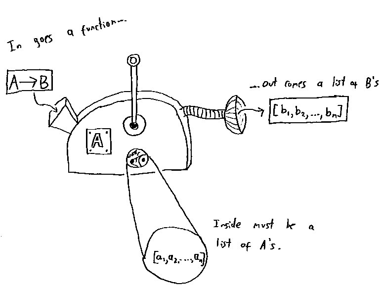
"But what about this..." you ask, suggesting an alternative definition for the machine:

> machine2' :: forall b . (a -> b) -> [b]
> machine2' f = reverse $ map f a where a = …to be determined…

That has the correct type signature but it doesn't seem to have the same form as machine2. However, with a tiny bit of work we can show it's functionally equivalent to one that does. In fact we can just plug machine2' into uncheck2 and it will give us a list of A's that can be used in machine2. Instead of reverse we could use any function [a] -> [a] and we'd still get a sensible result out of check2. The reason is that if f is of type forall a.[a] -> [a] then f $ map g a equals map g $ f a. (This is a Theorem for Free!.) So we can rewrite machine2' as

> machine2'' :: forall b . (a -> b) -> [b]
> machine2'' f = map f a where a = reverse $ …to be determined…

which looks just like our machine2. So however we munge up our list to make our machine unlike machine2 we can always 'commute' the munging to the right so it acts on the internal list of A's, converting into a machine like machine2.

One last example:

This time we hand our machine a A -> B and it gives us back another function, but this one is of the type C -> B, for some fixed C. It modifies the 'front end' of the input function so it can take a different argument. How could that possibly work? There's one obvious way: internally the machine is storing a function C -> A and when you hand it your function it returns the composition with the function it's storing.

Here's a potential design for this machine:

> machine3 :: forall b . (a -> b) -> (c -> b)
> machine3 f = f . a where a x = …to be determined…

Maybe you think there's another type of machine that converts A -> B's to C -> B's. If you do, try writing it. But I think there isn't.

So now we can write the code to reverse engineer machine3:

> uncheck3 :: (forall b . (a -> b) -> (c -> b)) -> (c -> a)
> uncheck3 t = t id

> check3 :: (c -> a) -> (forall b . (a -> b) -> (c -> b))
> check3 a f = f . a

uncheck3 pulls extracts the internally represented c -> a and check3 makes a functionally equivalent machine out of one.

So...I hope you're seeing the pattern. To make it easier, I'll define some functors:

> data I a = I a
> instance Functor I where
>    fmap f (I a) = I (f a)

> instance Functor ((->) a) where
>   fmap f = (.) f

Now all three example machines have the same form. For some functor f they map a function A -> B to an object of type f B and we deduce that internally they contain an f A. We can now write out versions of check and uncheck that work for all three machines:

> check :: Functor f => f a -> (forall b . (a -> b) -> f b)
> check a f = fmap f a

> uncheck :: (forall b . (a -> b) -> f b) -> f a
> uncheck t = t id

The above examples follow when we consider the functors I, [] and ((->) c) (for various values of c) respectively.

Yoneda's lemma is essentially the statement that check and uncheck are mutual inverses. So if you understand my examples, then you're most of the way towards grokking the lemma.

At this point I should add some details. We're working in the category of Haskell types and functions Hask. Expanding out the category theoretical definition of a natural transformation, t between two functors f and g in Hask gives t . fmap f == fmap g . t. In this category, natural transformations correspond to polymorphic functions between functors with no funny stuff so this equality actually comes for free. (To be honest, I haven't seen a precise statement of this, but it's essentially what Theorems for Free! is about.) Yoneda's lemma actually says that for all functors f there is an isomorphism between the set of natural transformations of the type forall b . (a -> b) -> f b and the set of instances of f a. So now I can give proofs:

uncheck (check f)
   = (check f) id        [defn of uncheck]
   = fmap id f           [defn of check]
   = id f                [property of fmap]
   = f                   [defn of id]

check (uncheck f) a
   = check (f id) a        [use defn of uncheck]
   = fmap a (f id)       [use defn of check]
   = f (fmap a id)       [f natural]
   = f (a . id)          [defn of fmap for ((>>) a)]
   = f a                 [property of id]

I'll confirm that check f is natural, ie. that (check f) . (fmap g) = (fmap g) . (check f), although, as I mentioned above, this is automatically true for polymorphic functions without funny stuff.

check f (fmap g x)
   = fmap (fmap g x) f   [defn of check]
   = fmap (g . x) f      [defn of fmap for ((->) a)]
   = (fmap g . fmap x) f [property of fmap]
   = fmap g (fmap x f)   [defn of (.)]
   = fmap g (check f x)    [defn of check]
   = (fmap g . check f) x  [defn of (.)]

So that's it, Yoneda's lemma. It's trivial because the isomorphism is implemented by functions whose implementations are a couple of characters long. But it's hard because it took me ages to figure out what it was even about. I actually started with examples outside of Haskell. But Haskell has this weird property that polymorphic functions, with minor restrictions, are natural transformations. (I think this is the deepest mathematical fact about Haskell I've come across.) And as a result, Hask is an excellent category in which to learn about Yoneda's lemma.

I also recommend What's the Yoneda Lemma all about? by Tom Leinster. His presheaf example is the one at which these ideas started making sense to me - but that's because I've spent a lot of time playing with Čech cohomology on Riemann surfaces, so it might not work for everyone. This comment is also worth some thought. In fact, is the Yoneda lemma itself a Theorem for Free?

I haven't said anything about the deeper meaning of the Yoneda lemma. That might have something to do with the fact that I'm only just getting the hang of it myself...

And if you're still confused, let me quote the ubiquitous John Baez: "It took me ages to get the hang of the Yoneda lemm[a]". And nowadays he's one of the proprietors of the n-Category Café!

NB Everything I've said is modulo the equivalence of natural transformations and polymorphic unfunny functions. I may have got this wrong. If so, someone please correct me as I'm sure everything I say here will still hold after some minor edits :-)

---

[1] Consider the following compiled using GHC with -fallow-overlapping-instances -fglasgow-exts:

> class Test a where
>     f :: a -> a

> instance Test a where
>     f = id

> instance Test Int where
>     f x = x+1

f is the identity for everything except for objects of type Int. This is an example of what I call "funny stuff".

[2] The accent on this letter 'č' is called a caron or háček. The book from which I learned about the Yoneda lemma used the caron to indicate the function I call check. I called it that because the TeX command to produce this symbol is \check. This is a multilayered pun, presumably by Knuth. It could just be that 'check' is an anglicised abbreviation for háček. But it's also a characterisically Czech accent so it's probably also an easier (for English speakers) spelling for 'Czech'. And I think it's also a pun on Čech. The caron is used on an H to represent Čech cohomology and so it's also called the 'Čech' accent. (I hope you can read those characters on a PC, I wrote this on a Mac.)

---

Variable substitution gives a...

...monad, of course. I keep telling myself that I'll write a post on topology or history of mathematics or something and then I end up saying something about Haskell monads. It seems to have happened again.

Anyway, it suddenly dawned on me that there's a monad to be wrung out of any recursive data structure. Roughly it goes like this: take a tree-like type, Tree a with some leaves are of type a. Visualise, if you will, an object of type Tree (Tree a), ie. a tree with leaves are themselves trees. You can graft the leaves that are trees directly into the parent tree giving you a Tree a. So grafting gives you a map Tree (Tree a) -> Tree a. That should remind you of part of the definition of a monad - this is the function called join in Haskell, or μ by category theorists. Note, for example, that grafting grandchildren into children before grafting the children into their parents gives the same result as grafting the children before the grandchildren. These, and other similar observations, give the usual monad laws.

Enough talk. Here's an expression datastructure.

> data Expr b = (Expr b) :+ (Expr b)
>                 | (Expr b) :* (Expr b)
>                 | F (Expr b) (Expr b)
>                 | I Int
>                 | V b deriving (Eq,Show)

Think of V b as a variable whose name is of type b. These are the points at which we'll graft in the subtrees. In this case, grafting will be the well known operation of substituting the value of a variable for the variable.

Here are the definitions:

> instance Monad Expr where
>     return b = V b
>     (a :+ b) >>= f = (a >>= f) :+ (b >>= f)
>     (a :* b) >>= f = (a >>= f) :* (b >>= f)
>     F a b >>= f = F (a >>= f) (b >>= f)
>     I i >>= f = I i
>     V b >>= f = f b

To apply >>= f you recursively apply it to the children except for V b where you actually get to apply f. So now we can define an 'enviroment' mapping variable names to values and construct an example tree e:

> env "a" = I 1
> env "b" = V "a" :+ I 2
> env "c" = V "a" :+ V "b"

> e = V "c" :+ I 3

It should be easy to see that e >>= env substitutes the value of c for V "c". But it's more fun to write this as the slightly bizarre looking:

> subst1 env e = do
>     a <- e
>     env a

> test1 = subst1 env e

We can read "a <- e" in English as "drill down into e setting a to the name of each variable in turn". So this is a backtracking monad like [] with a taking on multiple values. But notice how it only does one level of substitution. We can do two levels like this

> subst2 env e = do
>     a <- e
>     b <- env a
>     env b

> test2 = subst2 env e

With each line we drill down further into e. But of course we really want to go all the way:

> subst3 env e = do
>     a <- e
>     subst3 env (env a)

> test3 = subst3 env e

And so now I can confess about why I wrote this post. subst3 looks like a non-terminating loop with subst3 simply calling itself without ever apparently checking for termination, and yet it terminates with the correct result. Well I found it mildly amusing anyway.

Anyway, this >>= is a generalised fold meaning there's an F-algebra lurking around. Armed with the words F-algebra, monad and tree I was able to start Googling and I found this which points out that the connection between trees and monads is "well known".

Oh well, I've got this far, I may as well finish the job. That paper is about dualising the above construction so I'll implement it. This time, instead of considering trees where each node is optionally replaced by a label, we now have trees where every node has a label as well as a subtree. We call these labels decorations. In this case I think I'll work with trees are hierarchical descriptions of the parts of something (in a vain attempt to pretend this stuff is actually practical :-)

> class Comonad w where
>    counit :: w a -> a
>    cobind :: (w a -> b) -> w a -> w b

> data Parts' a = A [Parts a] | S String deriving (Eq,Show)
> data Parts a = P (Parts' a,a) deriving (Eq,Show)

> instance Comonad Parts where
>    counit (P (_,a)) = a
>    cobind f z = case z of
>        P (S s,a) -> P (S s,f z)
>        P (A l,a) -> P (A $ map (cobind f) l,f z)

We'll consider parts of a plane. We'll decorate the parts with their price. The function total computes the total price of a tree of parts. cobind now extends total so that every part is (unfortunately, inefficiently) redecorated with its total price including that of its subparts. If you're having trouble visualising comonads, this seems like a nice elementary example to think about.

> total (P (S _,n)) = n
> total (P (A x,_)) = sum $ map total x

> lwing = P (S "left wing",1000000)
> rwing = P (S "right wing",1000000)
> cockpit = P (S "cockpit",2000000)
> fuselage = P (S "fuselage",2000000)
> body = P (A [fuselage,cockpit],undefined)
> plane = P (A [lwing,rwing,body],undefined)

> test4 = cobind total plane

Uustalu and Vene's paper is pretty scary looking for something that's ultimately fairly simple!

Anyway, one last thought: this paper points out that in some sense, all monads and comonads can be thought of as trees with substitutions or redecoration.

Update: Modified the date of this entry. Blogger defaults to the day you first create an entry, not the date you publish. Let's see how many things break by fixing it to today...

The Poincare Conjecture on the Radio

I just thought I'd quickly mention that Melvyn Bragg has again chosen mathematics as the subject matter for his Radio 4 programme In Our Time. This time it's on the Poincaré conjecture. Again I'm amazed. Given that this is a series about all aspects of human culture, I think mathematics is actually being well represented. Downloadable as an mp3 from the BBC web site or through iTunes as a podcast.

Monads, a Field Guide

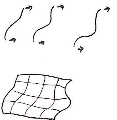
Here are some sketches of monads. I've annotated each with its species. I'm not a great artist and I only saw each of them for a fleeting moment so I had to fill in some details from memory. But I think the sketches are good enough to be able to recognise them in the wild. Click on the 'thumbnail' for the full size image.

I'm currently trying to stalk some monads from the continuation family. When I succeed I'll add some sketches of those too.

Games, Strategies and the Self-Composition of the List Monad.

Haskell is so strict about type safety that randomly generated snippets of code that successfully typecheck are likely to do something useful, even if you've no idea what that useful thing is. This post is about what I found when I tried playing with the monad¹ ListT [] even though I had no clue what purpose such a monad might serve.

I've talked about using monad transformers a couple of times. One time I looked at compositions of various types of side-effect monad, and more recently I looked at compositions of the List monad with side-effects monads. So it was inevitable that I got onto composing the List monad with itself to get ListT [].

This is literate Haskell, modulo the unicode characters.

So start with the the ordinary List monad, which is all about considering choices. For example the expression

> import Data.List
> import Control.Monad.Writer
> import Control.Monad.List

> test1 = do
>   x <- [1,2,3]
>   return (2*x)

> go1 = test1

can be interpreted as a program that chooses x to be each of the values 1, 2 and 3 in turn, applies f to each one and collects up the result to give [2,4,6]. The List monad will happily make choices within choices. So the expression

> test2 = do
>   x <- [1,2]
>   y <- [3,4]
>   return (x,y)

> go2 = test2

considers, for each possible choice of x, each possible choice of y. The result is [(1,3),(1,4),(2,3),(2,4)]. More generally, for fixed sets a,b,...c the expression

do
  x <- a
  y <- b
  …
  z <- c
  return (a,b,…,c)

returns the cartesian product a×b×…×c. In the fully general case, a,b,…c could all depend on choices that were made earlierbut right now I'm talking about the case when a,b,…,c are all 'constant'.

Here's a slightly different way of looking at this. Suppose a person called Player (P for short) is playing a solitaire game. At the first turn, P chooses a move from the set of possible first moves, then chooses a possible move from the set of second moves and so on. We can see that if we write the code

do
  move1 <- possible_moves_1
  move2 <- possible_moves_2
  …
  last_move <- possible_last_moves
  return (move1,move2,…,last_move)

the result is a list, each of whose elements is the sequence of possible plays in the game. If the possible_*; are all 'constant' then its just the cartesian product of the plays at each turn. But it's straightforward to adapt this code to enumerate all possible plays in a more general solitaire game - and that's exactly how the List monad is sometimes used to solve such games.

So if List is about making choices, composing List with itself might seem to be about making two types of choice. And the most familiar situation where you need to iterate over two possible types of choices comes when you consider two player games. So I'll tell you a possible answer now: ListT [] is the game analysis monad!

Let's look at some examples of code in the ListT [] monad. As I pointed out earlier, we use lift a when we want a to be a list in the inner monad and mlist a when we want a to be a list in the outer monad. So in ListT [] we can expect to use both of these with lists. Consider

> mlist :: MonadPlus m => [a] -> m a
> mlist = msum . map return

> test3 = do
>   a <- lift [1,2]
>   b <- mlist [3,4]
>   return (a,b)

> go3 = runListT test3

The value is [[(1,3),(1,4)],[(2,3),(2,4)]]. There's a nice interpretation of this. Introduce a new player called Strategist (S for short). Think of lift as meaning a choice for S and mlist as a choice for P. We can read the above as: for each first play a that S could make, go through all the first plays b that P could make. What's different from the solitaire example is how the plays have been grouped in the resulting list. For each decision S could have made, all of P's possible plays have been listed together in a sublist. But now consider this expression:

> test4 = do
>   b <- mlist [3,4]
>   a <- lift [1,2]
>   return (b,a)

> go4 = runListT test4

We get: [[(3,1),(4,1)],[(3,1),(4,2)],[(3,2),(4,1)],[(3,2),(4,2)]]. Maybe you expect to see the same result as before but reordered. Instead we have a longer list. Our interpretation above no longer seems to hold. But actually, we can salvage it?

Go back to thinking about solitaire games. We can read the code for test2 as follows: First choose a value for x, ie. x=1. Now choose a value for y, ie. y=3. Put (1,3) in the list. Now backtrack to the last point of decision and choose again, this time y=4. Put (1,4) in the list. Now backtrack again. There are no more options for y so we backtrack all the way back to a again and set x=1, and now start again with y=3, and so on.

Now we can reconsider test4 in a two player game. Think about the choices from the point of view of working through all of P's options while fixing one particular set of choices for S. (It took me a while to get this concept so I'll try to explain this a few different ways.) So P chooses b=3 and then S makes some choice, say a=1. Now we backtrack to P's next option, b=4. But on backtracking to P's last choice we backtracked through S's choice and on running forward again, we must make some choice for S, say a=1 again. There were 2 ways P could have played, so we end up with two distinct sequences of plays: (3,1) and (4,1) after P has worked through all of his options. We have a list with two possibilities: [(3,1),(4,1)]. But S could have played differently. In fact, because we play S's move twice for each sequence of P's moves there are three other ways this sequence could have come out, depending on S's strategy: [(3,1),(4,2)], [(3,2),(4,1)] or [(3,2),(4,2)]. And that is exactly what test4 gave: for each strategy that S could have chosen we get a list of all the ways P could have played against it. We get a list of 4 lists, each of which has two elements. Each of those elements is a sequence of plays.

I'll try to make precise what I mean by 'strategy'. By strategy we mean a way of choosing a move as a function of the moves your opponent has made. That's what we mean by a program t play a game: we give it a set of inputs and it then responds with a move. Its move at the nth turn is a function of everything you did for the previous n-1 turns. So consider the example above. After P has chosen from [3,4], S must choose from [1,2]. So S's strategy can de described by a function from [3,4] to [1,2]. There are 4 such functions. Once we've fixed S's strategy, there are 2 possible ways S can play against it. Again, we have 4 strategies, and 2 plays for each strategy.

And here's another way of looking at this. We'll go back to simple games where the set of options available at each stage are constant and independent of the history of the game. Let <A,B> mean a game where A is the set of S's strategies and B is the set of ways P can play against those strategies. (The set B doesn't depend on S's choice from A because we're now limited to 'simple' games.) Now introduce a binary operator * such that <A,B>*<C,D> is the game where the moves start off being those in <A,B> but when that's finished we move onto <C,D>. In <A,B>*<C,D>, P's options are simply B×D. So we know that in some sense <A,B>*<C,D>=<X,B×D> for some X. Now S's first move is from A so that bit's easy. S's second move from C depends on P's move from B. So S's second move is described by a function from B to C. So <A,B>*<C,D>≅<A×C^B,D>. (I use ≅ because I mean 'up to isomorphism'. C^B×A also describes S's strategies equally well.) * is a curious binary operation. It might not look it, but it's associative (up to ismorphism). And it has a curious similarity to the semidirect product of groups. Anyway, we can write test4 using this notation. It's computing <[1],[3,4]>*<[1,2],[1]> (up to isomorphism). [1] is just a convenient way of saying "no choice" and it gives us a way to allow P to move first my making S's first move a dummy one. Multiplying gives <[1,2]^[3,4],[3,4]>. [1,2]^[3,4] has 4 elements. So again we have 4 strategies with two ways to play against each of those strategies.

It's interesting to look at <A,B>*<C,D>*<E,F>. This is <A×C^B,B×D>*<E,F> which is <A×C^B×E^B×D,B×D×F>. This has a straightforward explanation: S gets to choose from A directly, to choose from C depending on how P plays from B and to choose from E depending on how P plays from both B and D.

And yet another way of looking at things. Suppose S and P are going to play in a chess tournament with S playing first. Unfortunately, before setting out on the journey to the tournament S realises he’s going to be late and is going to be unable to communicate during the journey. What should S do? A smart move would be to email his first move to the tournament organisers before leaving on the journey. That would buy him time while P thinks of a response. Even better, S could additionally send a list of second moves, one for each move that P might take in his absence. Going further, S could send a list of third moves, one for each of the first two moves that P might take in his absence. These emails, containing these lists, are what I’m calling a strategy. When you enumerate a bunch of options in the ListT [] monad you end up enumerating over all strategies for S and all responses for P.

It appears there’s a kind of asymmetry. Why are we considering strategies for S, but plays for P? This is partly explained by the above paragraph. In ListT [] there is an implicit ordering where S’s moves are considered to be before P’s. So if one of S’s choices comes after P’s, it needs to be pulled before P’s and that can only happen if it’s replaced with a strategy. There’s also another interesting aspect to this. When considering how to win at a game, you don’t need to test your strategy against every possible strategy your opponent might have. You only need to test it against every possible way your opponent could play against it and they only need to find one play to show your strategy isn’t foolproof. So ListT [] describes exactly what you need to figure out a winning strategy for a game.

Anyway, that’s enough theory. Here an application. The following code computes a winning strategy in the game of Nim. (If you don’t know Nim, then you’re in for a treat if you read up on it here. The theory is quite beautiful, but I deliberately don't use it here.) It uses brute force to find a winning strategy for S and additionally outputs a proof that this is a winning strategy by listing all possible ways the game could play out. Note that I’m using the WriterT String (ListT []) monad so I can log the moves made in each game.

I've also added another game, a variant of Kayles that I call Kayles'. In Kayles' there are n skittles in a row. On your turn you knock over a skittle and whichever of its immediate neighbours are still standing. The winner is the person who knocks over the last skittle. (The code describes the rules better than English text and you can adapt the code easily to play on any graph.)

Evaluate nim or kayles' to get a display of a winning strategy and a proof that it wins ie. a list of all possible games against that strategy showing they lead to P losing.

> strategies moves start = do
>  a <- lift $ lift $ moves start
>  tell $ [a]
>  let replies = moves a
>  if replies==[] then return () else do
>    b <- lift $ mlist $ replies
>    tell $ [b]
>    strategies moves b

> nim = mapM print $
>  runListT $ execWriterT $ strategies moves start
>  where
>  start = [2,3,5]
>  moves [] = []
>  moves (a:as) = [a':as | a' <- [0..a-1]]
>    ++ [a:as' | as' <- moves as]

> kayles' = print $ head $
>  runListT $ execWriterT $ strategies (kmoves (nbhd verts)) verts
>  where
>  kmoves nbhd v = [v \\ nbhd i | i <- v]
>  verts = [1..13]
>  nbhd verts i = intersect verts [i-1,i,i+1]

For example nim starts [[[2,3,1],…]] because a move to piles of size 2, 3 and 1 is a win in Nim. (2⊕3⊕1=0 for those who know the theory.) kayles' starts [[[1,2,3,4,5,9,10,11,12,13],…]] which means a winning move is to knock down skittles 6, 7 and 8 (you may see why symmetry makes this an obvious good opening move).

DISCLAIMER: I'm not claiming this is a good algorithm for solving games. Just that it illustrates the meaning of ListT [].

Finally a question. Are all monad transformers a form of semidirect product?

Footnotes:

[1] I haven't worked out the details but ListT [] probably isn't actually a monad. But it's close enough. It's probably associative up to ordering of the list, and as I'm using List as a poor man's Set monad², I don't care about ordering. An alternative ListT is provided here. I'm not sure that solves the problem.


[2] I'm pretty sure Set can't be implemented in Haskell as a monad. But that's another story.

Negative Databases

Protecting Data Privacy through Hard-to-Reverse Negative Databases is an entertaining paper. Here's the problem it tries to solve: You want to store personal details but you don't want people to be able to mine the database. For example you might want to store brief personal details with a social security number so you can verify that someone is a member of some organisation, but for security reasons you don't want a hacker to be able to get a list of members even if they steal the entire database. That sounds like an impossible set of requirements. But the trick is this: instead of storing the personal details you store a list of all possible bitstrings representing personal details that members don't have. Insane right?

If the personal details are just 256 bits long, say, then to store details for 100 people, say, the database needs 2²⁵⁶-100 entries. That's vast. But the database of non-members is highly compressible. Let me lift an example directly from the papers. Suppose the personal information is three bits long and we wish to store the entries {000,100,101}. Then the non-entries are {001,010,011,110,111}. The non-entries can now be compressed using a wildcard scheme {001,*1*}. The *1* represents all of the entries fitting that pattern from 010 to 111. This turns out to be quite a compact representation. It's beginning to look plausible.

And here's the neat bit: SAT can be translated into the problem of finding valid database entries from the wildcard representation. So extracting entries is provably NP-complete, despite the fact that we can check entries in a reasonable amount of time (for suitable definitions of 'reasonable').

Anyway, I still have a whole slew of objections, and the actual compression scheme proposed has holes in it that can result in false positives. But what initially sounded implausible is beginning to look workable.

PS You can also read about this at the Economist but I've tried to spare you the irrelevant fluff :-)

Infinitesimal Types

<mad thought>I want to combine two things I've previously discussed: Synthetic Differential Geometry (SDG) and Derivatives of Containers.

SDG is all about working with values, d, such that d²=0. When this is true, we find that for suitable functions f,

f(x+d)=f(x)+d f'(x)      (Eq. 1)

where f' is the derivative of f.

Now consider derivatives of types. I've written a really sloppy description here but for a proper treatment there are papers like this one. The curious idea is that if you 'differentiate' the type of a container you find the type of the container with a hole in it. Here's a really quick example: let F[X] be the container that is a triples of X's. In other words F[X]=X×X×X=XXX=X³. Here × is the usual product in the category of types. By a container with a 'hole' we mean a container with one of its elements missing, but with a 'hole' left behind so we know where the element has gone missing from. Consider the triple. Either the first element is missing. In this case there are two elements left, so we have something of type X². On the other hand the middle element could be missing, and the remaining elements also give something of type X². Or the last element could be missing. Put these three cases together and we get X²+X²+X²=3X². (The '3' in 3X² indicates that we know which of the three elements has been replaced with a hole.) If we use the prime symbol to mean differentiation we see that a triple with a hole in it is just dX³/dX=F'[X]. This generalises to other types, you can read the papers for more details. I think that's the most amazing bit of computer science I've seen in years. And it's even more fun with recursive types because you then get zippers.

Anyway, those are my ingredients and the following assumes that the above makes some kind of sense to you. So the mad thought I had was this: if you can do calculus by introducing infinitesimals such that d²=0, can we investigate containers with holes by introducing some kind of infinitesimal type with the bizarre property that

D²=0?
D is a type here, not a value. I'm hoping you can just play along here. Clearly we're talking about a weird kind of product when the product of a non-trivial object with itself is the zero object. Presumably to make sense of this we're not really talking about the usual categorical product, just as in the algebra R[d]/(d²) we're not talking about the usual real number multiplication. And note, of course, that I'm not saying that D is the type of infinitesimal numbers - I'm saying that the type itself is in some sense infinitesimal.

So what could D²=0 possibly mean? Well 0 is the type defined by the property that there are no values of type 0. So D²=0 simply means that you can't have a pair of objects of type D. So D isn't so weird at all, it corresponds to a type representing the singleton pattern. (Don't confuse this with the 'singleton' type 1. There is only one object of type 1 but we can have as many of them as we like. On the other hand, there may be many values an object of type D could take, but only one of those possible values can be realised.)

So now consider the type F[X+D]. This is a container, each of whose elements are of type X or of type D. Consider the case that they're all of type X. Then we have something of type F[X]. Now suppose that one of the elements is of type D. Then what we have is an F-container of X's with a hole, with a D in the hole. In other words, D×F'[X]. And now's the fun bit - this is all of the possible cases because the container can only contain one D. After all only one D can exist. Writing this out formally we get:

F[X+D]=F[X]+D F'[X]
In other words, we have interpreted Equation 1 in the context of types. As d can be thought of an infinitesimal value it makes sense to call D an infinitesimal type. I'm not sure how far you can run with this idea, but given that the argument above seems to make some kind of sense I expect a smarter person than me could give it rigorous form.

A final thought: D²=0 isn't really all that weird. We're already familiar with linear types and linear logic where we have things that can't be duplicated. This is just a different language to say something similar. Anyway, </mad thought>

You can fire me, but you can't stop me working!

In my last post I had a diagram consisting of a circle and a line tangent to it. I produced this using Grapher.app which comes with MacOS X, though unless you have a good look in /Applications/Utilities you might not realise it exists. This is the latest incarnation of Apple's graphing calculator. All I had to do was plot the graphs of y=0 and x²+(y-1)². And while it's a neat little application, what's really cool about it is the story of how it came into existence. It's an old story now, but lots of people still seem not to have heard it. It was developed illicitly, on Apple property, using Apple equipment, by an unpaid ex-Apple contractor who simply refused to leave. And despite the fact that he had to dodge his way around building security, and his project didn't show up on any official documentation, he managed to get resources allocated to his project and ultimately sneak his app onto the master disk image containing the release build of MacOS for the Power PC!



You can either read the full version of the story here or, and this is the version I recommend, you can listen to the programme from This American Life.

Update: Ron Avitzur contacted me to point out that Grapher is a separate application to Graphing Calculator. But I presume that Apple intended Grapher to be a followup to Graphing Calculator. Graphing Calculator is still being developed and I'll be playing with both apps now.

Practical Synthetic Differential Geometry

Previously I've talked about Automatic Differentiation (AD). My own formulation of the technique is more algebraic than the description that is usually given, and recently it's begun to dawn on me that all I've done is rediscover Synthetic Differential Geometry (SDG). I've looked at a variety of SDG papers but none of them seem to make the connection with AD. This is a pity because SDG allows you to do an amazing thing - write computer programs that easily manipulate objects such as vector fields and differential forms on manifolds without doing symbolic algebra. My goal here is to illustrate how the definition of vector field in Anders Kock's book gives a nice functional definition of a vector field and how that definition leads naturally to the Lie bracket. Normally it takes a significant amount of mathematical machinery to define these things but in the framework of SDG it becomes very simple. (Unfortunately this is going to be very sketchy as there's a lot I could say and I only have a small amount of time while I sit at home waiting for a new TV to be delivered...)

Kock's work is based on the idea of infinitesimal numbers whose square is zero but which aren't themselves zero. Clearly we aren't talking about real numbers here, but instead an extension to the real numbers. Here's a toy implementation:

> data Dual a = D a a deriving (Show,Eq)

> instance Num a => Num (Dual a) where
>   fromInteger i = D (fromInteger i) 0
>   (D a a')+(D b b') = D (a+b) (a'+b')
>   (D a a')-(D b b') = D (a-b) (a'-b')
>   (D a a')*(D b b') = D (a*b) (a*b'+a'*b) 

> e = D 0 1

They're called dual numbers because this particular algebra was apparently first described by Clifford and that's what he called them. The important point to note is that e^2==0. We can use the fact that

f(x+e)=f(x)+ef'(x)

to compute derivatives of functions. For example if we define

> f x = x^3+2*x^2-3*x+1

and evaluate f (1+e) we get D 1 4. We can directly read off f(1)=1 and f'(1)=4.

But, as Kock points out, the dual numbers don't provide 'enough' infinitesimals, we just get one, e, from which all of the others are built. So we can replace Dual with a new class:

> infixl 5 .-
> infixl 5 .+
> infixl 6 .*
> infixl 6 *.

> data R a = R a [a] deriving Show

> zipWith' f l r [] [] = []
> zipWith' f _ r a [] = map (flip f r) a
> zipWith' f l _ [] b = map (f l) b
> zipWith' f l r (a:as) (b:bs) = (f a b) : zipWith' f l r as bs

> (.+) :: Num a => [a] -> [a] -> [a]
> (.+) = zipWith' (+) 0 0

> (.-) :: Num a => [a] -> [a] -> [a]
> (.-) = zipWith' (-) 0 0

> (.*) :: Num a => a -> [a] -> [a]
> (.*) a = map (a*)

> (*.) :: Num a => [a] -> a -> [a]
> (*.) a b = map (*b) a

> (.=) :: (Eq a,Num a) => [a] -> [a] -> Bool
> (.=) a b = and $ zipWith' (==) 0 0 a b

> instance (Eq a,Num a) => Eq (R a) where
>    R a a' == R b b' = a==b && a'.=b'

A slightly more extended version of the Num interface:

> instance Num a => Num (R a) where
>    fromInteger a = R (fromInteger a) []
>    (R a a') + (R b b') = R (a+b) (a'.+b')
>    (R a a') - (R b b') = R (a-b) (a'.-b')
>    (R a a') * (R b b') = R (a*b) (a.*b' .+ a'*.b)
>    negate (R a a') = R (negate a) (map negate a')

And some more functions for good measure:

> instance (Num a,Fractional a) => Fractional (R a) where
>    fromRational a = R (fromRational a) []
>    (R a a') / (R b b') = let s = 1/b in
>        R (a*s) ((a'*.b.-a.*b') *. (s*s))

> instance Floating a => Floating (R a) where
>    exp (R a a') = let e = exp a in R e (e .* a')
>    log (R a a') = R (log a) ((1/a) .* a')
>    sin (R a a') = R (sin a) (cos a .* a')
>    cos (R a a') = R (cos a) (-sin a .* a')

The d i provide a basis for these infinitesimals.

> d n = R 0 (replicate n 0 ++ [1])

We now have an infinite set of independent dual numbers, d i, one for each natural i. Note that we have (d i)*(d j)==0 for any i and j. Apart from this, they act just like before. For example

f(x+d_i)=f(x)+d_if'(x).

We can use these compute partial derivatives. For example consider

> g x y = (x+2*y)^2/(x+y)

Computing g (7+d 0) (0+d 1) gives R 7.0 [1.0,3.0] so we know g(7,0) = 7, g_x(7,0)=1 and g_y(7,0)=3.

I'll use R as mathematical notation for the type given by R Float. (I hope the double use of 'R' won't be confusing, but I want to be consistent-ish with Kock.)

Before we do any more calculus, consider the following geometric figure:



A point is in the intersection of the circle and the line if it satisfies the equations:

> onS (x,y) = x^2+(y-1)^2==1
> onL (x,y) = y==0

Notice that in R this has many solutions. In fact, we find that onS (a*d 1,0) && onL (a*d 1,0) gives True for any Float value a. Does this mean anything? Actually, it fits some people's intuition of what the intersection should look like better than the usual idea that there is only one intersection point. In fact, Protagoras argued that there was a short line segment in common between the circle and the line and that because Pythogoras's theorem gave only one solution the whole of geometry was at fault! Using R instead of the reals makes sense of this intuition. The points of the form (a*d 1,0) do, indeed, form a line tangent to the circle. In fact, there is a way to construct tangent spaces and vector fields directly from this - but instead I want to now consider Kock's construction which is slightly different.

Let D be the subset of R consisting of numbers whose square is zero. These numbers are in some sense infinitesimal. In differential geometry a vector field is intuitively thought of as an 'infinitesimal flow' on a manifold. A finite flow on a manifold, M, is simply a function f:R×M→M such that f(x,0)=0. In f(x,t) we can think of t as time and each point x on the manifold flows along a path t→f(x,t). If f is differentiable, then as t becomes smaller, the path becomes closer and closer to a short line segment which we can draw as a vector. So the intuition is that a vector field is what you get in the limit as t becomes infinitesimal. The catch is that infinitesimal things aren't first class objects in differential geometry (so to speak). You can use infinitesimals for intuition, and I suspect almost all differential geoneters do, but actually talking about them is taboo. In fact, the definition of vector field in differential geometry is a bit of a kludge to work around this issue. When most people first meet the definition of a vector field as a differential operator it comes as quite a shock. But we have no such problem. In fact, Kock defines a vector field simply as a function

f:D×M→M

such that f(0,x)=x.
In the language of SDG, a vector field is an infinitesimal flow. For example, consider

> transX d (x,y) = (x+d,y)

This simply translates along the x-axis infinitesimally. Of course this code defines a flow for non-infinitesimal values of d, but when considering this as a vector field we're only interested in when d is infinitesimal. transX defines a vector field that everywhere points along the x-axis.

For those familiar with the usual differential geometric definition of vector fields I can now make contact with that. In that context a vector field is a differential operator that acts on scalar functions on your manifold. In our case, we can think of it acting by infinitesimally dragging the manifold and then looking at what happens to the function that's dragged along. In other words, if we have a funtion, f, on the manifold, the vector field v, applied to f, is that function vf such that f (f d x)==f x + d*vf x. For example with

> h (x,y) = x^2+y^2

h (transX (d 1) (1,2)) == R 5 [2] because h(x,y)=5 and h_x(x,y)=2.

I think I have enough time to briefly show how to define the Lie bracket in this context. If you have two vector fields, then intuitively you can view the Lie bracket as follows: take a point, map it using the first field by some small parameter d1, then map it using the second for time d2, then doing the first one by parameter -d1, and then the second by -d2. Typically you do not return to where you started from, but somewhere 'close'. In fact, your displacement is proportional to the product of d1 and d2. In other words, if your fields are v and w, then the Lie bracket [v,w] is defined by the equation v (-d2) $ v (-d1) $ w d2 $v d1 x==vw (d1*d2) x where vw represents [v,w]. But you might now see a problem. The way we have defined things d1*d2 is zero if d1 and d2 are infinitesimal. Kock discusses this issue and points out that in order to compute Lie brackets we need infinitesimals whose squares are zero, but whose product isn't. I could go back and hack the original definition of R to represent a new kind of algebraic structure where this is true, but in the spirit of Geometric Algebra for Free I have a trick. Consider d₁=1⊗d and d₂=d⊗1 in R⊗R. Clearly d₁²=d₂²=0. We also have d₁d₂=d⊗d≠0. And using the constructor as tensor product trick we can write:

> d1 = R (d 0) [] :: R (R Double)
> d2 = R 0 [1] :: R (R Double)

Let's test it out. Define three infinitesimal rotations:

> rotX d (x,y,z) = (x,y+d*z,z-d*y)
> rotY d (x,y,z) = (x-d*z,y,z+d*x)
> rotZ d (x,y,z) = (x+d*y,y-d*x,z)

Note that there's no need to use trig functions here. We're working with infinitesimal rotations so we can use the fact that sin d=d and cos d=1 for infinitesimal d. It is well known that [rotX,rotY]=rotZ and cyclic permutations thereof. (In fact, these are just the commutation relations for angular momentum in quantum mechanics.)

We can write

> commutator d1 d2 f g = (g (-d2) . f (-d1) . g d2 . f d1)

> test1 = commutator d1 d2 rotX rotY
> test2 = rotZ (d1*d2)

and compare values of test1 and test2 at a variety of points to see if they are equal. For example test1 (1,2,3) == test2(1,2,3). I don't know about you, but I'm completely amazed by this. We can get our hands right on things like Lie brackets with the minimum of fuss. This has many applications. An obvious one is in robot dynamics simulations where we frequently need to work with the Lie algebra of the group of rigid motions. This approach won't give us new algorithms, but it gives a very elegant way to express existing algorithms. It's also, apprently, close to Sophus Lie's original description of the Lie bracket.

I have time for one last thing. So far the only manifolds I've considered are those of the form Rⁿ. But this stuff works perfectly well for varieties. For example, the rotations rotX, rotY and rotZ all work fine on the unit sphere. In fact, if T is the unit sphere define

> onT (x,y,z) = x^2+y^2+z^2==1

Notice how, for example, onT (rotY (d 1) (0.6,0.8,0))==True, so rotY really does give an infinitesimal flow from the unit sphere to the unit sphere, and hence a vector field on the sphere. Compare this to the complexity of the traditional definition of a vector field on a manifold.

Kock's book also describes a really beautiful definition of the differential forms in terms of infinitesimal simplices, but I've no time for that now. And I've also no time to mention the connections with intuitionistic logic and category theory making up much of his book (which is a good thing because I don't understand them).

PS The D⊗D trick, implemented in C++, is essentially what I did in my paper on photogrammetry. But there I wasn't thinking geometrically.

(I don't think I've done a very good job of writing this up. Partly I feel horribly constricted by having to paste back and forth between two text editors to get this stuff in a form suitable for blogger.com as well as periodically having to do some extra munging to make sure it is still legal literate Haskell. And diagrams - what a nightmare! So I hit the point where I couldn't face improving the text any more without climbing up the walls. What is the best solution to writing literate Haskell, with embedded equations, for a blog?)

Local and global side effects with monad transformers

There is an annual puzzle event that 90 or so people attend. Each designs a puzzle and manufactures 90 copies of it which are then shared with the other participants. All 90 then get to go home with 90 puzzles.

Anyway, an ex-coworker attends this event and I had a chance to play with his puzzle. It was one of those fitting blocks together types puzzles. It was ingeniously designed but it seemed pretty clear to me that it required a lot of combinatorial searching. So I decided to write a program in Haskell to solve it using the List monad to enable simple logic programming.

But my code had a slight problem. It worked through the puzzle and found solutions, but (1) it didn't log the steps it took to achieve those solutions and (2) I couldn't count how many combinations it searched to find the solutions. Both of these could be thought of as side-effects, so the obvious thing to do is use a monad to track these things. But there was a catch - I was already using a monad - the List monad. When that happens there's only one thing for it - using a monad transformer to combine monads.

There are two distinct ways to combine a monad with the List monad and I needed both.

Anyway, this is literate Haskell. I'll assume you're vaguely familiar with using the List monad for logic programming. I also assume you're familiar with MonadPlus though that's not something I've written about here. And I couldn't get this stuff to work in Hugs, so use ghc. Here's some code:

> import Control.Monad.List
> import Control.Monad.State
> import Control.Monad.Writer

I'm not going to describe the original puzzle now. Instead I'm going to look at an almost trivial logic problem so that we can concentrate on the monad transforming. The puzzle is this: find all the possible sums of pairs of integers, one chosen from the set {1,2} and the other from the set {2,4}, where the sum is less than 5. Here's a simple implementation.

> test1 :: [Integer]

> test1 = do
>     a <- [1,2]
>     b <- [2,4]
>     guard $ a+b<5
>     return $ a+b

> go1 = test1

Run go1 and you should get the result [3,4]. But that's just the sums. What were the pairs of integers that went into those sums? We could simply return (a,b,a+b), but in more complex problems we might want to log a complex sequence of choices and that would entail carrying all of that information around. What we'd like is to simply have some kind of log running as a side effect. For this we need the Writer monad.

If you cast your mind back, monad transformers layer up monads a bit like layers of onion skin. What we want is to wrap a List monad in a Writer monad. We do this using the WriterT monad transformer. All we have to do is add a tell line to our code, and use 'lift' to pull the items in the list monad out from one layer of onion. Here's what the code looks like:

> test2 :: WriterT [Char] [] Integer

> test2 = do
>     a <- lift [1,2]
>     b <- lift [2,4]
>     tell ("trying "++show a++" "++show b++"\n")
>     guard $ a+b<5
>     return $ a+b

To get the final result we need to use runWriterT to peel the onion:

> go2 = runWriterT test2

Execute go2 and we get a list of pairs of sums and logged messages.

There's an important point to note here: we have one log per sum, so the logs are 'local'. What if we want a 'global' side effect such as a count of how many combinations were tried, regardless of whether they succeded or failed? An obvious choice of monad to count attempts is the State monad, but to make its effects 'global' we now need to make State the inner monad and make List provide the outer layer of skin. We're wrapping the opposite way to in the previous example. And now there's a catch. We use a line like a <- [1,2] to exploit the List monad. But now we no longer have a List monad, instead we have a ListT (State Integer) monad. This means that [1,2] is not an object in this monad. We can't use 'lift' either because the inner monad isn't List. We need to translate our lists into the ListT (State Integer) monad.

We can do slightly better, we can translate a list from the List monad into any other instance of MonadPlus. Remember that return x :: [X] is the same as [x] and x ++ y is the same as x `mplus` y :: [X]. For example [1,2] == (return 1) `mplus` (return 2). The latter only uses functions from the MonadPlus interface to build the list, and hence it can be used to build the equivalent of a List in any MonadPlus. To mplus a whole list we use msum leading to the definition:

> mlist :: MonadPlus m => [a] -> m a
> mlist = msum . map return

As a function [a] -> [a], mlist is just the identity. Now we're ready to go:

> test3 :: ListT (State Integer) Integer

> test3 = do
>     a <- mlist [1,2]
>     b <- mlist [2,4]
>     lift $ modify (+1)
>     guard $ a+b<5
>     return $ a+b

> go3 = runState (runListT test3) 0

Run go3 to see the result. Note we had to lift the modify line because the State monad is the inner one.

And now we have one more problem to solve: bouth logging and counting simultaneously:

> test4 :: WriterT [Char] (ListT (State Integer)) Integer

> test4 = do
>     a <- lift $ mlist [1,2]
>     b <- lift $ mlist [2,4]
>     tell ("trying "++show a++" "++show b++"\n")
>     lift $ lift $ modify (+1)
>     guard $ a+b<5
>     return $ a+b

> go4 = runState (runListT $ runWriterT test4) 0

That's it!

We can carry out a cute twist on this. By swapping the innermost and outermost monads we get:

> test5 :: StateT Integer (ListT (Writer [Char])) Integer

> test5 = do
>     a <- lift $ mlist [1,2]
>     b <- lift $ mlist [2,4]
>     lift $ lift $ tell ("trying "++show a++" "++show b++"\n")
>     modify (+1)
>     guard $ a+b<5
>     return $ a+b

> go5 = runWriter $ runListT $ runStateT test5 0

go5 returns a local count of how many combinations were required for each problem, and the Writer monad now records every 'try' in one long log.

One last thing: you don't need to explicitly 'lift' things - the monad transformers have a nice interface that automatically lifts some operations. (You may need a recent Haskell distribution for this, it fails for older versions.)

> test6 :: WriterT [Char] (ListT (State Integer)) Integer

> test6 = do
>     a <- mlist [1,2]
>     b <- mlist [2,4]
>     tell ("trying "++show a++" "++show b++"\n")
>     modify (+1)
>     guard $ a+b<5
>     return $ a+b

> go6 = runState (runListT $ runWriterT test6) 0

It'd be cool to get rid of the mlist too. Maybe if the Haskell parser was hacked so that [1,2] didn't mean 1:2:[] but instead meant (return 1) `mplus` (return 2) like the way Gofer interprets list comprehensions in any monad. (For all I know, Gofer already does exactly what I'm suggesting.)

One thing I should add - these monad transformers really kill performance. The puzzle solver I wrote no longer gives me any solutions in the few minutes that it used to...

PS I just made up the mlist thing. There may be a better way of doing this that I don't know about. I was surprised it wasn't already in the Control.Monad library somewhere. mlist is kind of a homomorphism between MonadPlusses and I think it might make the List MonadPlus an initial object in some category or other - but that's just speculation right now.

Update: I fixed the non-htmlised <'s. I think it takes more time to convert to blogger-compatible html than to write my posts! Also take a look at this. My mlist corresponds to their liftList - and now I know I wasn't completely off the rails writing mlist.

More Low Cost Geometric Algebra

In my second last post I showed how large algebraic structures could be built out of smaller ones using parametric polymorphism. In fact, for certain types, the type constructor acts like a tensor product in the category of algebras. It turns out that many of these structures are isomorphic to each other and Haskell provides a nice way to talk about these isomorphisms.

Before that I should say a bit more about Clifford algebras. These are an important tool in many branches of mathematics - algebraic topology, K-theory, representation theory and in theoretical physics. But one interesting aspect is that they can provide an alternative to the usual vector language of geometry. Many people will be familiar with the use of quaternions to represent 3D rotations. Clifford algebras generalise this to N-dimensions.

Before proceeding, note the footnote below on notation. And rather than write literate Haskell I've put the code here.

Back on topic: the first isomorphisms I should mention are

A⊗B≅B⊗A

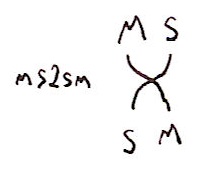
for any A and B. For example H⊗R(2)≅R(2)⊗H. As Haskell types this says that Quaternion (Matrix a) is isomorphic to Matrix (Quaternion a). Or in English: the 2×2 matrices of quaternions are isomorphic to the quaternions whose components are 2×2 matrices. This isn't completely trivial. For example let ms2sm be the isomorphism

ms2sm :: (Num a) => Matrix (Split a) -> Split (Matrix a)
ms2sm (M (S a b) (S c d) (S f g) (S h j)) =
    S (M a c f h) (M b d g j)

You can see that it's a little like a matrix transpose operation.

We can draw this pictorially as:


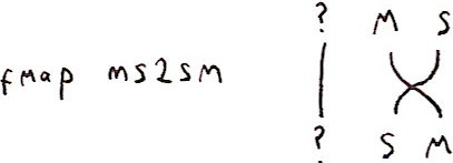
Note that the same function, because it is polymorphic, also gives an isomorphism Matrix (Split (Quaternion a)) -> Split (Matrix (Quaternion a)). But what about the isomorphism Quaternion (Matrix (Split a)) -> Quaternion (Split (Matrix a))? We can get this almost for free using the functoriality of the constructors. The isomorphism is fmap ms2sm. We can illustrate this as:

If we implement each of the pairwise flips then in combination with fmap we can get any permutation of the constructors. And you can probably imagine some pretty braid-like diagrams describing the process. (I could mutter something about symmetric monoidal categories here.)

These isomorphisms are almost trivial - they just swap elements around. But pick up any book that discusses Clifford algebras and you'll find a bunch of extra isomorphisms listed:

C⊗C≅C⊕C

C⊗H≅C(2)

H⊗H≅R(4)

For example, a quaternion of quaternions is much the same as a 4×4 matrix. We choose to represent the latter as a 2×2 matrix of 2×2 entries with the isomorphism

qq2mm :: (Num a) => Quaternion (Quaternion a) -> Matrix (Matrix a)
qq2mm (Q (Q a b c d) (Q f g h j) (Q k l m n) (Q p q r s)) =
    M (M (a+g+m+s) (b-f-n+r)  (f-b-n+r)  (a+g-m-s))
      (M (c+j-k-q) (d-h+l-p)  (h-d+l-p)  (c+j+k+q))
      (M (j-c+k-q) (d+h+l+p)  (-d-h+l+p) (j-c-k+q)
      (M (a-g+m-s) (-b-f+n+r) (b+f+n+r)  (a-g-m+s))

(That took me a few minutes of actual work to unpack the proof of that in Spin Geometry by Lawson and Michelson so it's no longer for free!) There's a really important reason why you might want to do this. It takes 16 multiplications of the underlying elements to multiply two quaternions but it only takes 8 multiplications to multiply 2×2 matrices. A Matrix (Matrix a) can therefore be multiplied four times as fast as a Quaternion (Quaternion a). So being able to switch back and forth between repesentations is useful.

I think I now have a simple kit of parts for manipulating Clifford algebras efficiently. If I have time I should try to write a complete library for N-dimensional Clifford algebras. I wonder if I could apply it to path counting methods?

Back to isomorphisms. I want to mention two in particular. One is

C_n+8=R(16)⊗C_n

The actual isomorphism is

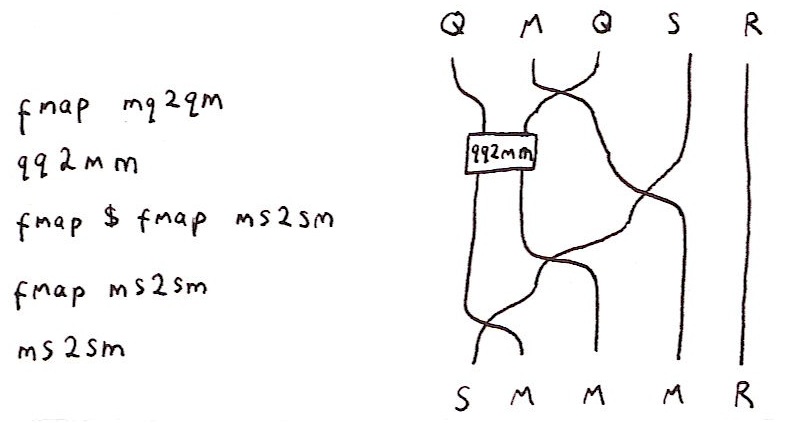
bott :: Num a => Quaternion (Matrix (Quaternion (Matrix a))) -> Matrix (Matrix (Matrix (Matrix a)))
bott = qq2mm . fmap mq2qm

It's prettier viewed pictorially:


As I've mentioned before, this isomorphism is an example of Bott periodicity. It pops up in many places in mathematics, for example in Supergravity or K-Theory.

This is an interesting isomorphism:

Remember that Split a is essentially a pair of objects of type a. So we can define

cliff72left,cliff72right :: Cliff7 -> Matrix (Matrix (Matrix R))
cliff72left = first . ms2sm . fmap ms2sm . (fmap (fmap ms2sm)) . qq2mm . fmap mq2qm
cliff72right = second . ms2sm . fmap ms2sm . (fmap (fmap ms2sm)) . qq2mm . fmap mq2qm

This gives not one, but two different ways to represent an element of C₇ as an 8×8 matrix. But there's more to it than that. The main real-world application for quaternions is for describing rotations - they're well used in the 3D graphics world for example. Elements of C₇ can be used to describe rotations in 8D. (Modulo a sign ambiguity that should be familiar to anyone who's played with quaternions.) So what he have is that a rotation in 8D can be represented with 3 different 8×8 matrices: the usual one, and the two coming from C₇ (modulo the sign). This has many implications in physics. For example these three matrices describe how bosons, left-handed fermions and right-handed fermions transform under rotations. In 8-dimensions these matrices are all 8×8 making 8D a special dimension for doing physics. By a roundabout path this is closely linked to the 10D of superstring theory. This "theewayness" is known as triality which John Baez has written about a few times.

I'm getting to like this type constructor as tensor product viewpoint. I can see a lot of mathematics that be expressed nicely in it. General relativity and knot theory are two that come to mind...

Footnote about notation

I go back and forth between conventional mathematical notation and Haskell. I also have one letter abbreviations I use in function names and diagrams. The translation table is:

Mathematics	Haskell	Abbreviation
R⊕R	Split	s
C	Complex	c
H	Quaternion	q
R(2)	Matrix	m
Cn	CliffN
C'n	CliffN'

Learn Maths with Haskell

This is a quick plug for the web site of a friend of mine, David Amos. He's been working hard to produce a treasure trove of useful mathematical code in Haskell with the intention of making abstract objects more accessible to mathematics learners.

Highlights include code for

1. Commutative algebra, including Gröbner basis computation and tools for manipulating ideals of rings.
   
2. Permutation groups, including an implementation of the Schreier-Sims algorithm and tools for investigating the Rubik's cube group and its subgroups.
   
3. Number theory. Includes tools for working with quadratic fields, p-adic numbers and elliptic curves, and code for factoring using Lenstra's elliptic curve algorithm.
   

The full repository is here. (Use that link to download the code as some of the other links appear to be broken right now.)

It'd be great to see a textbook grow out of some of this work...

Geometric Algebra for Free!

I'm a fan of Haskell. But I'm not a zealot. I'll be the first to tell you that some of the stuff down below works better in C++. But C++ has syntax uglier than a mandrill's rear end so I'll sacrifice functionality for readability. This is literate Haskell by the way. Copy and paste this whole entry into a .lhs file and run it with hugs -98 or ghci -fglasgow-exts.

The first bit of functionality I'll sacrfice is some of the genericity of my code so let's start with fixing a base field. Everything I say below will be over the reals:

> type R = Float

Anyway, today's theme is about how writing your code generically allows you to combine classes together in unanticipated ways to give you useful stuff - more or less for free.

If you've done some mathematical coding you probably have a complex number class lying around somewhere. If it's written in a modern language it's probably generic allowing you to choose your base structure. For example in C++ you might be able to use complex<float> or complex<int>. If you don't have such a class you can have a Haskell one for free:

> data Complex a = C a a deriving (Eq,Show)

> instance Num a => Num (Complex a) where
>     fromInteger a = C (fromInteger a) 0
>     (C a b)+(C a' b') = C (a+a') (b+b')
>     (C a b)-(C a' b') = C (a-a') (b-b')
>     (C a b)*(C a' b') = C (a*a'-b*b') (a*b'+b*a')

The usual complex numbers are given by Complex R. But here's a question: does Complex (Complex R) mean anything. Complex a requires a to be a Num, but Complex R is a Num. So Complex (Complex R) compiles fine. But does it mean anything mathematically? It does, it corresponds to C⊗C. (Remember, I'm working over the reals, so by ⊗ I mean ⊗_R.) If you're shaky on tensor products then I can give a one line summary for the case of working over the reals: A⊗B means opening up the object of type A and replacing every occurence of a real number in it with a copy of a B. For example, a complex number can be thought of as an object that contains two real numbers. So C⊗C is an object that contains two complex numbers and which multiplies in a certain way. So the type constructor Complex actually corresponds quite well with the functor _⊗C. It's even better, if ⊗ is thought of as the tensor product in the category of algebras, not just vector spaces, then the Complex type constructor computes a tensor product of algebras. This is kinda obvious but I've never seen anyone say this explicitly. (Clearly the same is true of a C++ template like complex<>.)

So let's look at some examples. Maybe you also have a matrix class lying around. If you don't, here's a 2 by 2 matrix class for you:

> data Matrix a = M a a a a deriving (Eq,Show)

> instance Num a => Num (Matrix a) where
>     fromInteger a = M (fromInteger a) 0 0 (fromInteger a)
>     (M a b c d)+(M a' b' c' d') = M (a+a') (b+b')
>                                     (c+c') (d+d')
>     (M a b c d)-(M a' b' c' d') = M (a-a') (b-b')
>                                     (c-c') (d-d')
>     (M a b c d)*(M a' b' c' d') = M (a*a'+b*c') (a*b'+b*d')
>                                     (c*a'+d*c') (c*b'+d*d')

We can start putting our words into practice. Use the notation A(n) to mean the n by n matrices with entries in A. Then A(n)=R(n)⊗A. So the type constructor Matrix is the functor _(2). Another theorem is that R(m)⊗R(n)=R(mn). This means that Matrix (Matrix R) gives 4 by 4 matrices. Neat eh? We're already getting some classes for free. But we can get bigger stuff for free.

I'm also a fan of geometric algebra. But I'm not a zealot. Geometric algebra can do a lot of neat stuff but I'm not one of those people campaigning to get everyone to throw out their old vectors and tensors to replace them with geometric algebra.

Geometric algebra is all about Clifford algebras. The Clifford algebra, Cliff(n), is the real numbers extended by throwing in n elements e_i, for i from 1 to n, and all of the things you can get my multiplying and adding these numbers. In addition we impose the rules that e_i²=-1 and e_ie_j=-e_je_i. You already know some Clifford algebras. Cliff(0) is just r. Cliff(1) is C because i serves perfectly well as e₁. Cliff(2) is probably familiar to you as well, it's just the quaternions. Ah...but quaternions have three values whose square is -1, so surely it's Cliff(3). Well, no actually. e₁=i, e₂=j and k is reallly just ij, ie. e₁e₂, and so isn't something new. In general, Cliff(n) is 2ⁿ dimensional with a basis consisting of all of the possible products of the e_i. Anyway, if you don't already have a Quaternion class, here's one for you:

> data Quaternion a = Q a a a a deriving (Eq,Show)

> instance Num a => Num (Quaternion a) where
>     fromInteger a = Q (fromInteger a) 0 0 0
>     (Q a b c d)+(Q a' b' c' d') = Q (a+a') (b+b')
>                                     (c+c') (d+d')
>     (Q a b c d)-(Q a' b' c' d') = Q (a-a') (b-b')
>                                     (c-c') (d-d')
>     (Q a b c d)*(Q a' b' c' d') = Q (a*a'-b*b'-c*c'-d*d')
>                                     (a*b'+b*a'+c*d'-d*c')
>                                     (a*c'+c*a'+d*b'-b*d')
>                                     (a*d'+d*a'+b*c'-c*b')

There are also another bunch of Clifford algebras called Cliff'(n). Cliff'(n), is the real numbers extended by throwing in n elements e_i, for i from 1 to n. With the properties e_i²=1 and e_ie_j=-e_je_i. Note the 1 instead of -1. Cliff'(1) is known as the split complex numbers. You might not have an implementation of these, so here you go, gratis:

> data Split a = S a a deriving (Eq,Show)

> instance Num a => Num (Split a) where
>     fromInteger a = S (fromInteger a) (fromInteger a)
>     (S a b)+(S a' b') = S (a+a') (b+b')
>     (S a b)-(S a' b') = S (a-a') (b-b')
>     (S a b)*(S a' b') = S (a*a') (b*b')

You already have an implementation of Cliff'(2). Believe it or not, it's isomorphic to the 2 by 2 matrices. e₁=[[-1,0],[0,1]] and e₂=[[0,1],[1,0]], using the obvious Haskell lists to represent matrices. (Try squaring those matrices and seeing what you get.)

That's all well and good, but what about Cliff(n) for larger n. The obvious thing is to represent the elements as arrays of length 2ⁿ. But to multiply these things we'd have to loop over each element of the first multiplicand and then over each element of the second meaning a loop that takes time 2²ⁿ. But who wants to write code when you can get stuff for free? Check outh this paper on the classification of Clifford algebras. On page 5 there's an important theorem
Cliff(n+2)=Cliff(2)⊗Cliff'(n)
Cliff'(n+2)=Cliff'(2)⊗Cliff(n)
Now we know how to implement tensor products this becomes trivial. In Haskell notation,

> type Cliff1  = Complex R
> type Cliff1' = Split R
> type Cliff2  = Quaternion R
> type Cliff2' = Matrix R
> type Cliff3  = Quaternion Cliff1'
> type Cliff3' = Matrix Cliff1
> type Cliff4  = Quaternion Cliff2'
> type Cliff4' = Matrix Cliff2

and so on.

That's it. We've built Cliff(n) and Cliff'(n) out of a bunch of simple classes that you might already have had lying around. Geometric algebra for free! It almost seems sad to see a beautiful classification theorem demystified in such a simple way. Still, you don't see pairs of mutually recursive towers of types like this every day.

But actually this is all a con. It's no good having something isomorphic to what we want without the actual isomorphism. For example where is e₃ in Cliff4', say? So we now have to do a tiny bit of real work. Start with a type class:

> class Clifford b where
>     i :: R -> b
>     e :: Int -> R -> b

i is the function that embeds our base field, the reals. And e i a is intended to be ae_i.

And now we simply assert:

> instance Clifford R where
>     i a = a
>     e _ _ = error ""

> instance Clifford (Complex R) where
>     i a = C a 0
>     e 1 a = C 0 a

> instance Clifford (Split R) where
>     i a = S a a
>     e 1 a = S a (-a)

Now we can define i and e for all of the algebras. For the details look at the proof of Theorem 3.4. They translate almost directly as:

> instance (Num b,Clifford b) => Clifford (Quaternion b) where
>     i   a = Q (i a) 0 0 0
>     e 1 a = Q 0 (i a) 0 0
>     e 2 a = Q 0 0 (i a) 0
>     e n a = Q 0 0 0 (e (n-2) a)

> instance (Num b,Clifford b) => Clifford (Matrix b) where
>     i   a = let b = i a in M b 0 0 b
>     e 1 a = let b = i a in M (-b) 0 0 b
>     e 2 a = let b = i a in M 0 b b 0
>     e n a = let b = e (n-2) a in M 0 b (-b) 0

And now we really do have usable Clifford algebras. Here are some more defintions:

> type Cliff5  = Quaternion Cliff3'
> type Cliff5' = Matrix Cliff3
> type Cliff6  = Quaternion Cliff4'
> type Cliff6' = Matrix Cliff4
> type Cliff7  = Quaternion Cliff5'
> type Cliff7' = Matrix Cliff5
> type Cliff8  = Quaternion Cliff6'
> type Cliff8' = Matrix Cliff6
> type Cliff9  = Quaternion Cliff7'
> type Cliff9' = Matrix Cliff7

(In C++ you can define 'metafunctions' that map integers to classes. Doing something similar in Haskell is pretty ugly.)

And I've learnt my lesson from my monad tutorial. Here's a little test to make sure I'm actually telling the truth:

> t  i = e i 1 :: Cliff9
> t' i = e i 1 :: Cliff9'
> 
> test a t n = map (\(i,j) -> (t i)*(t j)+(t j)*(t i)==0) [(i,j) | i <- [1..n], j <- [1..(i-1)]] ++
>              map (\i -> (t i)*(t i)==a) [1..n]

> fulltest = and $ (test (-1) t 9) ++ (test 1 t' 9)

If fulltest evaluates to True then we know that for Cliff9 and Cliff9' we have created Haskell objects that satisfy the defining properties for e_i.

One last thing, let's consider the complexity of this code. The naive algorithm multiplies two elements of Cliff(n) in time O(2²ⁿ). It's an easy exercise to see that the multiplication time is O(2^7n/4). Not bad for something that was free. We can acualy do quite a bit better with some small changes - for example by using Strassen-like tricks for all but the Split multiplications.

But if you really want to do this stuff properly check out this paper which I haven't yet read properly.

I'd also like to add that Cliff(n+8)=R(16)⊗Cliff(n), so we have a kind of repeat with period 8. This is known as Bott periodicity and it lies at the heart of many of the most beautiful things in mathematics including some fascinating properties of the number 8.

---

Algebraic Topology in Haskell

On my shelf I have the book "Basic Topology" by Armstrong. After you've fought your way through 173 pages you eventually get to the section on simplicial topology and you can start playing with one of the basic tools of modern topology: homology groups. But you don't want to go through all that hassle. If you can read Haskell code then you can get there in 20 lines. But don't get too excited - this isn't meant to be an introduction to algebraic topology. Instead it's a demonstration of how incredibly expressive Haskell is. Before starting on this project I expected it to take a couple of weeks of early morning hacking and many hundreds of lines of code. It actually took a couple of hours.

So the goal is this: use the standard chain complex from simplicial homology to compute the Betti numbers.

First we need some code to compute the rank of a matrix. As this is general purpose code I'm not counting it in my 20 line budget. It took me a little while to find a recursive implementation of this suitable for Haskell. Basically, the idea is that a zero matrix has zero rank and the following operations leave the rank of a matrix unchanged:

1. Deleting a row of zeroes
   
2. Deleting a column of zeroes
   
3. Multiplying a row or column by a non-zero constant
   
4. Adding one row to another.
   

One last thing is needed: if there is a non-zero value standing on its own in a row or column then deleting both the row and column that it is in reduces the matrix rank by one. Here's the complete code for the rank function:

import List

rank m = let m' = removeZeroRows $ removeZeroColumns m in
    if m'==[]
        then 0
        else let (zero,(pivot:rest)) = break ((0 /=) . head) m' in
            1+rank (map (cancelZero pivot) (zero++rest))
    where
    removeZeroColumns x = let n = foldl1 min (map countZeros x) in
                            map (drop n) x
    removeZeroRows = filter (or . map (0 /=))
    countZeros = length . fst . break (0 /=)
    cancelZero (a:as) (b:bs) = zipWith (\x y -> a*y-b*x) as bs

With that out of the way, here is the code to compute the homology of a simplicial complex:

d x = zip (d' x) (cycle [1,-1]) where
    d' [] = []
    d' (x:xs) = xs : (map (x:) (d' xs))

matrix basis1 basis2 op = map (coefficients basis1 . op) basis2 where
    coefficients basis x = map (flip coefficient x) basis
    coefficient e = sum . lookup e
    lookup k [] = fail ""
    lookup k ((k',v):xs) = if k == k' then return v else lookup k xs

grade n = filter ((==(n+1)) . length)

dim c = foldl1 max (map length c)-1

dmatrix _ 0 = []
dmatrix c n = matrix (grade (n-1) c) (grade n c) d

betti c = let d = dim c
              ranks = map rank $ map (dmatrix c) [0..d]
              dims = map (\i -> length (grade i c)) [0..d] in
              h dims ranks where
              h (c:cs) (d:d':ds) = c-d-d' : h cs (d':ds)
              h [c] [d] = [c-d]

That's it! No hundred thousand line algebra library, or polygonal mesh geometry library. Just the standard Haskell List library.

At this point I suggest looking at something like these notes on simplicial complexes. My d function corresponds to ∂ defined at the bottom of page 1.

Let's take the example at the bottom of page 2 and the top of page 3:

example = [
    [1,2,3],
    [1,2],[1,3],[2,3],[2,4],[3,4],
    [1],[2],[3],[4],[5]]

(Note I don't have anything corresponding to F_-1. This is always the set containing the empty set so the code is hard coded to work as if it were there.) If you play with the dmatrix routine you'll see that it gives the matrices on page 3 (transposed).

And now we can fire up ghci or hugs and get:

*Main> dmatrix example 1
[[-1,1,0,0,0],[-1,0,1,0,0],[0,-1,1,0,0],[0,-1,0,1,0],[0,0,-1,1,0]]
*Main> betti example
[2,1,0]

The example has 2 connected components, 1 1-hole, and no 2-holes. (Quick one line summary of the whole of algebraic topology: Make a hole in a piece of paper: that's a 1-hole. Hollow out the interior of a solid sphere: that's a 2-hole, etc.)

Here are some more topological spaces to play with:

point = [[0]]
line = [[0],[1],[0,1]]
ball n = sublists [0..n] \\ [[]]
sphere n = ball (n+1) \\ [[0..(n+1)]]
torus = [[1],[2],[3],[4],[5],[6],[7],[8],[9],
    [1,2],[2,3],[1,3],
    [5,9],[8,9],[5,8],
    [4,6],[6,7],[4,7],

    [1,5],[4,5],[1,4],
    [2,9],[6,9],[2,6],
    [3,8],[7,8],[3,7],

    [1,9],[3,9],[1,8],
    [4,9],[6,8],[5,7],
    [1,6],[2,7],[1,7],

    [1,5,9],[1,2,9],[2,3,9],[3,8,9],[1,3,8],[1,5,8],
    [4,5,9],[4,6,9],[6,8,9],[6,7,8],[5,7,8],[4,5,7],
    [1,4,6],[1,2,6],[2,6,7],[2,3,7],[1,3,7],[1,4,7]]

The torus is copied from page 4 of the notes. Here are some more examples:

*Main> betti (sphere 3)
[1,0,0,1]
*Main> betti (sphere 0)               
[2]
*Main> betti torus
[1,2,1]

But that's not all. Pay your $19.95 right now and I'll throw in barycentric division for free:

sublists [] = [[]]
sublists (a:as) = let b = sublists as in b ++ map (a:) b

properSublists x = sublists x \\ [x]

chain f x = [x:xs| x' <- f x, xs <- chain f x'] ++ [[x]]

bary x = x >>= chain (filter (not . null) . properSublists)

As expected, barycentric division of a simplicial complex leaves the homology unchanged:

*Main> betti (bary torus)
[1,2,1]
*Main> 

OK, I admit, it's a little slow on the last one. But it does have to perform unoptimised Gaussian elimination on fairly large matrices. (Type dmatrix ((bary torus)) 2)

And here's my laundry list of things to do with this project:

1. More efficiency. The vectors over the simplices are stored incredibly inefficiently.
   
2. Compute homology groups over Z, not Q. I just use dimension counting to compute the dimensions of the homology groups over a Q. I really ought to actually compute the kernels of these matrices and then find representatives of the homology groups. I also need to write code to manipulate Abelian groups rather than vector spaces. To my shame, I don't know what the algorithms to use for the latter are.
   
3. Compute cohomology groups.
   
4. Compute homology groups associated to a poset. (The barycentric subdivision code kinda does this already.) Actually, this is where I started from originally. alpheccar asked if there was a connection between certain types of Hopf algebra and the Euler characteristic. I think the answer is yes: it comes from computing the Euler characterstic of posets used to define the Hopf algebra. Actually, the whole renormalisation with Hopf algebras thing that alpheccar points out is reminiscent of a really beautiful paper I read years ago on "fat graphs" that computes the Euler characteristics of the very moduli spaces used in string theory.
   

And the last thing on my list I can do right now. Computing the Euler characteristic, via the Betti numbers, is a one liner:

euler c = sum (zipWith (*) (betti c) (cycle [1,-1]))

Of course I showed there was an easier way to compute this earlier.

How can Haskell not be the programming language that all mathematicians should learn?

Update: I just found some slides on the "fat graph" thing I mentioned above. I rate it as one of the most beautiful pieces of mathematics ever. Some time I'll devote a whole post to it.

What can we measure? Part II

If you followed Part I then I should now be able to give an accessible lead in to some of the stuff John Baez has been talking about over the years.

So far I've illustrated examples of Hadwiger's theorem and showed how Hadwiger's 0-volume corresponds to the Euler characteristic (at least for certain finite unions of bounded shapes). Note how the r-volume has the dimensions of length^r meaning that the Euler characteristic is the only possible dimensionless quantity that is rotation- and translation-invariant and finitely additive. The Euler characteristic of a finite subset of Rⁿ is simply the cardinality of the subset. And because any kind of notion of cardinality probably ought to have the invariance properties I mention above, it looks like the Euler characteristic might provide a weird alternative to the usual notion of cardinality, despite the fact that it assigns the negative value -1 to the interval (0,1) in R. It certainly behaves a lot like cardinality and it has the additive property that you'd expect cardinality to have. It gets even better, it also have the right multiplicative property. In particular, for the kind of polyhedra objects I talked about in Part I, v₀(A×B)=v₀(A)v₀(A). But that's not all.

From now on I'll write the more usual χ instead of v₀. If you have two finite sets, A and B, then the set of functions from A to B is written B^A (at least if you're not a Haskell programmer). It's also standard stuff that for finite sets #(B^A)=#B^#A. Amazingly, if you compute the Euler characteristic in the right way, it makes sense to say that χ(B^A)=χ(B)^χ(A) for many other kinds of set too, despite the fact that χ(A) can now end up taking on negative, rational or even irrational values. χ is simply begging to be interpreted as an alternative way to count things!

If you take a peek at what Propp and Baez have to say about this you'll see that despite all of this tantalising evidence, there isn't yet a solid theory that says what any of this really means. In order to compute Euler characteristics, both Propp and Baez find themselves carrying out bizarre computations like

1+2+4+8+…=Σ_n=0…xⁿ (where x=2) =1/(1-x)=1/(1-2)=-1

(or these) which seem to give an Euler characteristic that's consistent with the other things that have been computed, and yet this computation, in itself, is nonsensical. It's clear that not only are we not sure how to answer the questions we can pose about the Euler characteristic, we're not even sure what the right questions are, or even what concepts we should be using. These are exciting times and I'm hoping that a slew of great mathematics should develop out of this over the years.

Anyway, to get back on topic. It's not just counting that's at issue, from the above summation we can see that the ordinary notion of the sum of a series is also problematic, in particular the notion of a sum of an infinite series. So let's think back to how we define such sums. We consider the sequence of partial sums and then take the limit - for every ε there is a δ such that.... In other words, to form such a limit we have to use ideas from metric spaces. So starting with an algebraic concept, the finite sum, we make the 'leap' to infinite sums by importing machinery from analysis. It's now so ingrained into us that despite the fact that ordinary summation is an algebraic concept, we understand the sum to mean a concept from analysis. But as Hadwiger's theorem shows, there are ways of making the leap to sums over infinite sets without using analysis. Conventionally we count the size of a structure by throwing away most of the structure so we're left with nothing but some underlying set, and then we use the fact that we already have a theory of cardinality for these bare sets. But what Baez & co. have been pointing out is that there seem to be alternative notion of cardinality that compute the size of something directly without throwing away the structure. We can go straight from object→number rather than going object→set→number. (Baez would say something about how we're working in a category other than Set.)

So why does this matter? Have a look at the beginning of these notes by Richard Borcherds. (Aside: I'm completely out of academic social circles these days so it's an utterly amazing coincidence that I bumped into him at a party a few weeks ago and he told me he was into QFT these days.) From the beginning it's dealing with the question of how to compute integrals that diverge. In QFT we compute the probability of something happening by summing over all of the possible ways it could happen. But this space of all possible ways is incredibly large - infinite dimensional in fact. Analysis fails us - as Borcherds points out on page 2, there is no Lebesgue measure on this space meaning we can't hope to perform this summation in the conventional way. Physicists end up having to perform nonsensical calculations just like the one above to get their answers. It seems like physicists are also using the wrong kind of summation. Maybe the Euler characteristic isn't just abstract nonsense but is actually the tool we ned in physics.

So here's my take on all this: the reason we use the sum to refer to a concept from analysis is that analysts were the first people to give a rigorous definition of an infinite sum. Maybe if a combinatorialist like Propp had got there first we'd be using a different notion. In particular, physicists all try to compute their sums in an analytic way and get into a mess as a result. The whole field of renormalisation is one horrific kludge to work around the fact that infinities crop up all the way through the work of physicists. Maybe we need to find a new way to count that doesn't throw away our underlying structures and so can give us sensible answers.

For example, consider bosonic string theory. (And by doing this I'm not in any way trying to endorse String Theory. I just happen to know some of the mathematics behind it. Physicists are very polarised over whether or not it's a good physical model, and just mentioning the field is enough for them to think you have joined one camp or another. It's just a good 'toy' model.) To get sensible answers we have to go through the usual shenanigans to get finite numbers. But there's a really neat parallel with Hadwiger's theorem. Just as insisting on rotation- and translation-invariance narrows down the possible notions of cardinality, in String Theory conformal-invariance pins down the possible ways we might sum over all paths. In fact, it pins things down so well that not only is there only one possible way to carry out our summation, it shows that this summation only makes sense in 26 dimensions. So what is this space we're summing over? Well as a string moves through space it sweeps out a surface called a worldsheet:

So we're looking at summing over the space of all possible 2D surfaces of a certain type. These are known as moduli spaces. In particular, if we want to sum over all of these surfaces, we must start by summing over all such surfaces with one loop in them, ie. sum over all toruses. We need to consider the space of all such toruses. Turns out there's a nice way of looking at this space. I won't spell out the details but the space looks like the shaded region below

folded up in a certain way. (The 'certain way' is described here.) The folded up space is an example of an orbifold. Each point in this space corresponds to one torus so every possible path that a string can take that sweeps out a surface with one 'hole' corresponds to one point in this space. And John Conway et al. have written a nice document on how to compute the Euler number of an orbifold and this one has an Euler characteristic of -1/12.

I'll come back to this in a moment. But there's another approach to String Theory. Again, I'm not going to any kind of detail. But part of the calculations require looking at the vibration modes of a string. Just like with a musical instrument you get a fundamental 'note' and higher overtones. When a quantum string string is in its lowest energy state it has some of its energy stored in each mode of vibration. If the lowest mode of vibration has 1 unit of energy, the first overtone has 2, the second has 3 and so on. So when we try to find the total energy of a string in its lowest energy state, part of the computation requires summing 1+2+3+4+…. It's one of these apparently meaningless sums but physicists can use a trick called zeta regularisation to get the result -1/12. It's the same number as above but arrived at in a completely different way.

So here's my theory about what's going on. (Unlike other people out there who are crackpots, I have the decency to warn you when I might be grossly misunderstanding other people or even making stuff up. :-) The problem is that physicists keep getting infinities because they have to compute these infinite sums. And they start to calculate these sums by 'creeping up on them', ie. by taking the limit as you compute each of the partial sums. They're trying to use the analyst's definition of summation using deltas and epsilons. Unfortunately, the things physicists are trying to sum over are so large there simply isn't a way to creep up on infinity like this. So instead, I think we have to redefine what we mean by counting and summation. Instead we should be using the Euler characteristic. The -1/12 above is a clue that this is the right track - because when physicists try to use their weird renormalisation tricks to get answers it's not unusual for the result to end up having a mysterious Euler number connection. So it's as if the weird tricks are just a shadow of some deeper kind of mathematics that one day will make sense. But we can't just sum over any old set in this way - there needs to be some other structure that tells us how to compute these sums. In the case of Hadwiger's theorem, if we assume the sums are dimensionless and invariant under rotations and translations then that is enough information to pin down precisely one possible meaning of the sum - the Euler characteristic. What John Baez and co. are doing is trying to find other kinds of structures that are relevant for physical theories and I'm hoping that one day these will lead to a new notions of summation that work for them.

I've drifted a bit from my original topic - a chapter in a course from a graphics convention, so I'll stop there. But here's the one paragraph summary of what I'm saying: just as we can count the elements in a set, there is also a notion of counting for other kinds of structure. We don't really have a proper theory of what this means but we do have some partial results that suggest the Euler characteristic is connected somehow. And maybe when we have a proper theory, and literally a new way to count, the problems with infinities that plague any kind of quantum field theory will go away.