Using markets to aggregate information

If you have a wide variety of sources of probabilistic information how do you aggregate it together? From the Microbe World podcast (if you're wondering - yes, I do listen to a regular podcast about microbes!) I learnt that people who need to predict outbreaks of flu have taken an interesting approach to this problem.

Researchers at the University of Iowa have set up an Electronic Market to allow experts in fields to trade on their beliefs. By observing how much people are prepared to bet on various outcomes we can get an aggregated expert opinion of how likely these outcomes are. Apparently they perform fairly well as predictors of the future. And one of these markets is the Influenza Prediction Market where you can buy stock in your favourite influenza strain.

On a related note, the Foresight Exchange has been running for many years now. Click on "claims" and select "Science & Technology:Math" to bet on the likelihood of the Collatz Conjecture or the Riemann Hypothesis.

"I love the Hahn-Banach Theorem"

No, not me. I'm just quoting:

I love the Hahn-Banach theorem. I love it the way I love Casablanca and the Fontana di Trevi. It is something not so much to be read as fondled.

Thus begins the abstract to the eulogy "On the Hahn-Banach Theorem" by Lawrence Narici.

There's not much I can add to that. Have you ever felt this way about a theorem?

(I have a virulent dislike of analysis but I'm going to see if this paper can convert me.)

What is a Saros?

Until recently I though that solar eclipse prediction involved quite a bit of celestial mechanics. Not so, it turns out you can get a pretty good handle on when eclipses are likely to occur just by considering the periods of various cycles and using a simple continued fraction approximation.

At any instant, the orbit of the Earth around the Sun lies in a plane. Clearly the Moon must lie in this plane for an eclipse to take place.

The orbit of the Moon around the Earth also lies in a plane. A different one, in fact. The intersection of these planes forms a line. The two points where this line meets the orbit of the Moon are known as nodes. In order to have a solar eclipse the Moon clearly must lie near a node.

As the moon orbits it travels from a node back to the same node in 27.21222 days (a draconic month).

A solar eclipse can only take place at a new moon. New moons take place every 29.53059 days (a synodic month).

Solar eclipses will take place each time the cycles of a half-draconic month (there are two nodes) and a synodic month coincide.

The ratio of the two periods is approximately 2.170391. So we can get an idea of when the cycles will coincide by constructing rational approximations to this ratio. We can use continued fractions to form them and one of these is 484/223. 242 synodic months is equal to 223 draconic months to within an hour and is equal to 6585 and a third days (approximately 18 years). This time interval is known as a saros.

So, if a solar eclipse has just taken place, then to a good approximation, we can expect another eclipse exactly one saros later. What's more, because a saros is 1/3 day, modulo a day, we know that the location of the subsequent eclipse will be 120 degrees longitude west. (Note that solar eclipses will happen more often than once a saros, but eclipses separated by a saros are interesting because they form a regular sequence, to a good approximation.)

But every rational approximation to the ratio given above will give some kind of approximate eclipse cycle, so why focus on the saros? The saros has another interesting property. The Moon's orbit is elliptical. This allows us to define another cycle: the time taken to move from major axis, to minor axis, to major axis again. This is the time period over which the Moon-Earth distance is periodic and is known as an anomalistic month. It turns out that that one saros is almost exactly 239 anomalistic months. When the Moon is closest to the Earth it looks bigger than the Sun and when it is furthest it looks smaller. This makes the difference between a total eclipse, where the Moon completely occludes the Sun, and an annular eclipse, where an annulus of the Sun is visible. Because a saros is close to an integer multiple of this period, solar eclipses separated by a saros are likely to be of the same type.

According to wikipedia this time period is named after a Babylonian word because the Babylonians were aware of this cycle. I'll believe that when someone tells me how the Babylonians knew that the eclipses were taking place one third of the way across the world.

Armed with this knowledge I must read how Stonehenge can be used to predict eclipses.

Do Particles Exist?

In quantum mechanics, the state of a particle is given by an element of a vector space - typically something like a Hilbert space. But what happens if you want to investigate multiple particles and the number of particles may change over time? Then you need to use quantum field theory. Suppose we're dealing with one type of particle. Then the state space now looks like

V=V₀⊕V₁⊕V₂…

Where vectors in V_n describe states with n particles.

Now, here I'm going to start getting out of my depth. But I'm sure people out there can correct my errors. And I'm treading dangerously by rephrasing things a little differently from how they appear in any of the books or papers I have read.

Each of these V_ns carries a representation of the Poincaré group. This means that if we apply a translation, rotation or boost to a vector in V_n we get another state V_n. So rotating, boosting or translating an n particle state just gives you another n particle state. The upshot of this is that all inertial observers can agree on how many particles a state represents.

But suppose now that we accelerate our state. We map our underlying spacetime with a function f so that if p(t) is the worldline of an inertial observer, f(p(t)) is now the worldline of an observer accelerating with constant acceleration, say a. f induces a linear mapping on V. The details of the computation are a bit messy but essentially what happens is that an n-particle state is now mapped to a state that is a linear combination of elements from all of the V_i. In particular, elements of V₀ end up mapping to states with particles. Let me quote Wikipedia

the very notion of vacuum depends on the path of the observer through spacetime. From the viewpoint of the accelerating observer, the vacuum of the inertial observer will look like a state containing many particles

These particles are called Unruh radiation. But I find this notion bizarre. How can the number of particles depend on the observer? And how does this look in practice? Well suppose we're in a vacuum and someone called Fred accelerates past with a particle detector. Fred's detector will start beeping to indicate the presence of particles even though I don't get any beeps with my detector. I will in fact see Fred's detector act like it's detecting particles. In other words, although Fred and I might disagree over how many particles occupy this region of space, we can both agree on what the detector is doing. This isn't a big deal at all, we're used to the idea of non-inertial instruments acting funny, just trying using a pair of scales in an accelerating car.

So here's my conclusion from all of this: either

1. It makes no sense to interpret the detection of particles by the accelerating detector as indicating that the vacuum contains particles. We can't trust the readings from a non-inertial particle detector without some kind of correction for acceleration. This is completely familiar, lots of other kinds of instruments fail when non-inertial. The actual definition of the number of particles in a region of space is chosen so as to correspond with what an inertial detector sees.
   
2. The notion of particle, separate from that of a detector, is meaningless. We just have a Hilbert space of states and instruments that go beep under certain circumstances and we can predict when these instruments go beep by looking at properties of the Hilbert space.
   

Most physicsts seem to use another option:

3. The number of particles depends on the frame of reference in which you are measuring
   

Anyway, things get even trickier. If you look at how V is split up into n-particle subspaces it turns out that the definition of this splitting depends on a choice of direction for time. In a flat spacetime we can pick any timelike direction because they're all basically related by Lorentz transforms so they all give the same results. But in a curved spacetime it's not so easy. Again we end up with an ambiguity in the number of particles, but this time (at least near a black hole) it's called Hawking radiation. I interpret this as meaning we have to take option 2. Particles simply aren't a well-defined concept, except as an approximation, in a curved spacetime. However, most physicsts still take option 3. I'm happy with option 2 because I see quantum mechanics as being primarily about vectors in a state space, not about particles. Physicists seem happy to take option 3 even though I think it's nonsensical. They're used to the idea of a quantity that is frame-dependentm eg. the x-coordinate of a vector, and feel that it's fine to extend this notion to integer valued properties such as particle number.

But what do I know? I'm not an expert in this field. I did try to study this field properly many years ago, eg. by reading Wald's book on black hole thermodynamics. I found it to be mostly clear, but I had many problems because I kept having objections to the physics, something I hadn't felt with any of the physics I had studied previously, including wacky stuff like renormalization.

Anyway, I don't have anything to contribute to this subject, I just thought I'd mention it because people might find it interesting. I discussed it a little bit with someone who knows a lot more about this subject over at Reality Conditions and I now have a bunch of papers to read on the subject. Unfortunately the setting for much of this work is C*-algebras and the like so I need to swot up on all that stuff first.

Iannis Xenakis and Formalized Music

John Baez recently sparked quite a bit of discussion of music and mathematics over on sci.physics.research. But nobody seems to have mentioned the composer that many see as the most rigorously mathematical of all: Iannis Xenakis. Born in Romania with Greek ancestry and eventually adopted by the French, Xenakis started his career as a civil engineer and architect and only later turned to music.

I have listened to three CDs by Xenakis: Music for Strings, Persepolis and Legende D'Eer. Out of these, Music for Strings is a collection of pieces that come closest to the usual notion of music in that notes are played at various pitches on conventional instruments. Probably the most distinctive features are the wild glissandi flying in all directions (to use a spatial metaphor). The other two discs consist of hour long pieces that sound superficially like unpleasant extended accidents in a junkyard.

I decided to try to find out in what way these works were mathematical. After much searching on the web I found a paper by Edward Childs describing part of Xenakis's stochastic composition process. Apparently Xenakis made explicit use of four probability distributions in the composition of a piece call Achorripsis. I'll concentrate on three of these as I believe there is a way to drastically simplify Childs's description of these while combining them into one single scheme.

Xenakis composed his piece by creating a grid of 28 columns and 7 rows. Each row represents a group of instruments and each column represents a time period. Xenakis created a number of musical events and stochastically assigned these to cells in the grid. Within each grid cell he also chose the pitch of each event and the timing between events using stochastic methods. In particular, he generated the number of events in a cell using a Poisson distribution, the timing between events using an exponential distribution and the pitch of events using a uniform distribution. This composition dates from 1957 and this prompted Childs to say

The preparation of the score was a remarkable feat considering
that he worked without the help of a computer, but
calculated all distributions, and their musical implementation,
by hand.

Now, suppose that Xenakis had taken his grid and pinned it up on the wall. If he then stood some distance from the grid, blindfolded (actually, Xenakis would only have needed an eye patch), and had thrown darts at the grid, what distributions would we see? If he was far enough away and blindfolded there'd be unlikely to be any kind of bias towards one part of the grid or another meaning that the darts that hit the grid would be uniformly distributed. The number falling in each cell would have a Poission distribution. The spacing between successive pairs of darts along a horizontal axis would have an exponential distribution, and the heights of each dart would be uniformly distributed. In other words, Childs's description is entirely consistent with Xenakis having generated a large part of his composition with darts, with a single dart simultaneously generating the three random variables desired. So much for formalized music.

Let me quote another composer, Pierre Schaeffer, quoted in Childs's paper:

As far as Xenakis is concerned, let me emphasize
at once that I’d be much more interested in his research
if he hadn’t set out so obviously to reduce its
accessibility and its credibility in a manner which is
immediately apparent as soon as you open his book
on formal musics.

Was Xenakis using mathematics to hide his composition methods from other, less mathematically savvy, composers?

Nonetheless, whatever his composition methods, after listening to Xenakis I seem to be finding other types of music to be far too clichéd and predictable. I think I have developed a liking for this composer. If you hear what seems to be the sound of pneumatic drills, thermal lances and scraping metal as you drive over the San Francisco Bay Bridge in the morning, look around, it might not be the bridge retrofit, but instead me commuting to work listening to one of Xenakis's electroacoustic works.

(PS If you're wondering, the fourth distribution, that I omitted, was the Maxwell-Boltzmann distribution, which Xenakis used to generate the speeds of the glissandi.)

Even More Numb3rs

There are so many blogs about the TV series Numb3rs out there, it hardly seems worth it for me to write about it myself, especially as it has now been renewed for its third season. But when I talk to my mathematical inclined colleagues, very few of them have actually watched the series. Mathematics on TV is so incredibly rare that I would have thought that they would jump at the chance to see a popular TV show with a high mathematical content. So clearly word isn't getting out and I'm going to talk about it anyway.

Numb3rs is yet another FBI series with the protagonists solving crimes. What makes it different is that Charlie, the brother of the lead FBI agent, is a mathematician who consults for the agency. What's astonishing about the series is that week after week, Charlie uses mathematics to solve crimes. He's a mathematical crime fighting superhero. What's more, I've watched most of the first series, and the mathematics used in each episode actually has a degree of plausibility.

You might not be convinced. So here's a quick summary of the plot of the pilot episode (on the DVD of season one):
<SPOILER>

Charlie tries to track a serial killer by fitting a probability distribution to the attacks, with the assumption that the killer lives at the 'centre' of the distribution. It fails to produce a lead. But then Charlie has the flash of inspiration that he should be looking for a bimodal distribution with two peaks. He reworks the data and finds both where the killer lives and where he works. This is prime time TV. 10pm Friday night (where I live). We have a TV show where the plot hinges on how many local maxima a probability density function has. I don't know about you, but I find this quite unbelievable. But amazingly, this is a real TV series.
</SPOILER>


The show isn't problem free. I'm not exaggerating when I describe Charlie as a superhero. He solves mathematical problems in a new field overnight that would take experts days, weeks or months. The editing is pretty choppy - we cut from scene to scene with rapid fire explanation leaving viewers without enough time to assimilate information. (Watching on DVD so you can rewind and pause helps.) The scripts feel a little like writing by numbers (so to speak). You feel a little too aware of when the writers have gone into "character development mode" or "action mode" or "explain for the benefit of the audience mode" and the character development is all standard stuff.

I have to say that I'm pretty impressed with the inventiveness of the writers in creating mathematics related plots. My dream job would be creating mathematical or scientific ideas for TV shows (I could have invented much better technobabble than Heisenberg compensators and there have been countless scripts that I'd have loved to have touched up.) But I doubt I could have created as many plots as the Numb3rs team have managed. And despite the exaggeration, they've done so without making the mathematics completely preposterous (at least not in the first season).

And one last quibble: does Charlie have to say "statistical analysis" and "equation" so often?

Laws of Form: An Opinion

I just reread George Spencer-Brown's Laws of Form. I mentioned this book a year ago but at that time I was talking from memory and from second hand descriptions. I finally got hold of a copy for around $20 and worked my way through it. You can find out about a little of the content here.

But after this rereading I think I'm now ready for the final verdict: is this a crackpot book or not?

Well - in the first few chapters it develops a kind of boolean algebra using 'forms' built out of Spencer-Brown's 'distinction' symbol. It's cute because he's constructing an algebra that has just the one symbol. Everything he has to say here seems more or less fine.

In the following chapters variables are introduced. It gets a little confusing. At first the variables are metavariables in the sense that they are used by Spencer-Brown to represent his forms. But later on he introduces variables within his system at which point we have something equivalent to propositional calculus. The earlier boolean style algebra can now be interpreted as a model for this calculus. But it's all very confusing because he doesn't make it clear when an expression is to interpreted in the algebra or the calculus. Nonetheless, he then proceeds to prove the kinds of theorems you'd expect a logician to prove, viz. soundness and completeness.

He then introduces imaginary values. This is the point at which I became lost in my first reading years ago. Interpreting the 'distinction' as boolean 'not', he's introducing a logical value that is a solution to x = not x. Clearly neither x=true nor x=false do the job so Spencer-Brown claims to introduce imaginary values that are solutions. It seems like a lot of nonsense, but in my second reading of the book it made perfect sense. I don't think that he says enough to completely disambiguate the meaning but I was able to provide an interpretation, in Haskell, that fits his description. Quite simply, the logical values in Spencer-Brown's system need to be interpreted as streams of boolean values, ie. as type [Bool]. The distinction operator (call it cross) can now be defined as

cross :: [Bool] -> [Bool]
cross a = False : map not a

In other words, it's just a not with a delay. But there is a catch, the text talks vaguely about a delay, but not what the initial value of the stream should be. So I actually define cross by

cross :: Bool -> [Bool] -> [Bool]
cross init a = init : map not a

and provide my own values of init as required by the context.

So how do I know this is the correct interpretation? Well the book contains a counter circuit that is supposed to take logical signals as inputs and output a signal that flips value half as often as the input. I was able to take his circuit and transcribe it directly into Haskell (making some choices of init values) and amazingly it performed exactly as described. (This tool goes further than my code, but it still has to deal with the ambiguity issue.)

Here's the code:

(#) = zipWith (||)
cross a = False : map not a
i = cross i
m = True : m
n = False : n
delay n x = replicate n False ++ x
pulse m = replicate m True ++ n

b0 = i
b1 = [False,False,True,True]++b1
b2 = [False,False,False,False,True,True,True,True]++b2

b n = replicate n False ++ map not (b n)

trace a = let b = take 120 a in
let t x = if x then "-" else " " in
putStr $ unlines [b >>= t,b >>= (t.not)]

gate a b = let f = cross (cross (f # a) # b) in f

nor init x y = init : map not (x # y)

count a = let b = nor False a f
c = nor True b d
d = nor False b j
e = nor False a h
g = nor False e j
h = nor False f c
j = nor True d e
f = nor True g h
in f

test = count $ map not $ (b 4)

main = do
trace (map not (b 4))
trace test

a # b means a written next to b. cross a means a inside a distinction or crossing. Instead of building the circuit using cross I use nor, corresponding to the shorthand GSB uses. The definition of count is neat. It's a mutualy recursive definition that essentially allows me to label various points in the circuit and wire them up. It's really amazing that Haskell allows you do do this. Anyway, run main and it'll draw the two 'oscilloscope' traces. (You'll need a w-i-d-e terminal window.) There's a brief discussion of the circuit here.

So, Laws of Form succeeds in defining a boolean style algebra and propositional style calculus. It then shows how to build circuits using logic gates. And that, as far as I can see, is the complete content of the book. It's fun, it works, but it's not very profound and I don't think that even in its day it could have been terribly original. (Who first proved NAND and NOT gates are universal? Sheffer? Peirce?) In my view this makes GSB's mathematics not of the crackpot variety, despite his talk of imaginary logical values.

But...GSB's style is classic crackpot stuff. His writing borrows more from the Tao Te Ching than from conventional mathematics texts. He uses delberately obfuscated language and makes pronouncements that read like the writings of mystics. It's no surprise that when there was a conference on GSB's work it took place at Esalen.

So my final opinion, for all of the two cents that it's worth, is that GSB is a little on the crackpot side, but that his mathematics in Laws of Form is sound, fun, cute, but, despite the trappings, not terribly profound.

k-calculus and Special Relativity

I've been familiar with Special Relativity since childhood - I think I was able to give Einstein's old trains and light rays argument for time dilation when I was barely out of elementary school. (Unfortunately my brain only went downhill from there...) So I was pretty surprised when I started reading Bondi's introduction to Relativity for the layman, Relativity and Common Sense, published in the fifties, and found that I was learning something new.

At one point in the book, Bondi shows that different observers, who appear to have synchronised watches, end up having watches showing different times. Amazingly he seems to do all of this in what looks like a Newtonian framework. It took me several rereadings of the paragraphs to eventually realise where it was that he'd sneaked in the relativity assumption. I felt like I'd just seen one of those puzzles where you rearrange a square as a rectangle which appears to have a lower area. But as a result of this, he makes Special Relativity seem like the most natural thing in the world. And the really nice thing is that in his presentation he doesn't need to talk about watches that use light pulses (because the sceptic might say that time dilation only applies to watches that use laser pulses) but instead his argument applies to any kind of watch.

Anyway, the key idea is this: suppose A and B have zero relative velocity. If A signals B at one minute intervals then B will receive the signals at one minute intervals. But if A and B move apart with constant velocity, B will receive A's signals less frequently simply because the signals have to cover an increasing distance as B moves from A. This much is trivial and applies to any non-instantaneous signal in a Newtonian or Einsteinian framework.

Now suppose B receives signals every k minutes. The key step is this: according to relativity, k can only be a function of the relative velocity of A and B, not a function of the absolute velocities of A and B. Using this assumption, and some other far less radical ones that few people would have problems with, the rest of Special Relativity follows. But you'll have to read the book for the details (or google for k-calculus).

It's all very elementary stuff. But this k-factor argument seems like it would be much more convincing to the layman than Einstein's original thought experiment. In fact, I did a bit of googling and it seems that the k-factor argument has been presented in a few different places under the name "k-calculus".

Bondi also stresses that watches are like odometers. They measure something that is personal to the path that you have taken rather than some absolute observer independent quantity. This is something that is hard to get from other elementary accounts I have read. Other introductions present time dilation as some kind of influence that somehow makes your clocks go 'wrong'. Just the name 'time dilation' gives the impression that what you measure is somehow dilated from the 'correct' time, a completely erroneous view. Just as there is no 'distance' dilation for driving north-east and then north-west to get to a place due north.

Anyway, if you have some doubting Thomas relative (no pun intended) who thinks the whole Relativity thing is bogus, but they do have a bit of numerical aptitude, this might be the book to get them. You don't even need to compute a square root to compute the discrepancy between the watches in Bondi's first example. All in all, an excellent book!

Anyway, my reason for reading this book is that I really don't like the way some physicists talk about Relativity. So I thought I'd read a few elementary accounts to get an idea of what trends there are in explaining the subject.

(Sadly, Bondi passed away last year. And maybe I've finally got over my resentment of Bondi for giving me low marks for the cosmology questions in exams at Cambridge one year...)

How to Divide by Three

I just came across this paper by Peter Doyle and John Conway (though it seems that Conway disowns it!).

Ostensibly it proves something simple: that if there a bijection from A×3 to B×3 (where 3 = {0,1,2}), then there is a bijection from A to B. The catch is that the authors choose not to use the axiom of choice and so must explicitly describe the bijection. It turns out this is a hard problem. Lindenbaum claimed a proof in 1926 but it was 'lost'. Tarski published a proof in 1949 but Conway and Doyle think their proof is probably a rediscovery of Lindenbaum's original.

It's very curious. A priori I'd never have guessed this was a tricky problem.

It seems that the ubiquitous John Baez mentioned this a hundred 'weeks' ago here. Does that man have to have already written on everything that interests me in mathematics!? :-)

A Taylor Series for Types

There's a result that I'm surprised isn't mentioned in Derivatives of Containers. It's pretty obvious considering what's in that paper but it's still interesting to mention, so maybe it's well known and too obvious for anyone else to state explicitly. Basically this

F[X+Y]=F[X]+Y F'[X]+Y²/2! F''[X]+Y³/3! F'''[X]+...

is true when interpreted as a statement about types.

But first I have to say what I mean by dividing a type by n!. That's explained at the end of the above paper, but first some notation: Let n be the set {0,...,n-1}. Then use the suggestive notation X! to mean the group of permutations of X. Clearly #(n!)=n!, where the on the right hand side I'm using ! to mean factorial. We now allow groups to act on containers by permuting the elements within them. For example a triple of X's is written X³. This datatype has a notion of an ordering of the elements ie. (1,2,3) is not the same as (3,2,1). The group 3! acts in a natural way on triples by permuting the three elements. If we take the quotient by this group then we get the 3-element bag where order doesn't matter. So Xⁿ/n! is the n-element bag. (As pointed out in the paper, we can't define sets in this way because sets require a notion of equality.)

The paper also shows that F'[X] is the type of F-containers with one of the X's punched out to leave a hole. So F⁽ⁿ⁾[X] is an F-container with n holes punched out. But note that it still retains information about the order in which the holes were punched out. For example, consider pairs with F[X]=X². F''[X]=2. This corresponds to the fact that there are two orders in which you can punch out the two elements of a pair.

Now consider a Yⁿ/n! F⁽ⁿ⁾[X]. This is an F-container of X's where n of the X's have been punched out, combined with n Y's. We can insert the n Y's into the holes in the order specified by the F⁽ⁿ⁾[X]. So Yⁿ/n! F⁽ⁿ⁾[X] is an F-container of X's with n of the X's replaced by Y's.

Now look at the right hand side of the Taylor series. This is basically an F-container of X's where some (or zero) of the X's have been replaced by Y's.

And finally note what the left hand side is: it's an F-container of X+Y's. Ie. each object in the F-container is either an X or a Y. And it's pretty obvious that's the same thing as a container of X's where some of the X's are replaced by Y's.

I like to write it as F[X+Y]=exp(Y d/dX)F[X].

Hey! I just discovered there's a Container Type blog!

Fun with Derivatives of Containers

This is a neat paper.

So more thinking out loud...

Consider functions that map streams of X's to streams of Y's. As streams are a linear ordering of elements we can label positions in the output stream using natural numbers starting at zero. So a function that maps streams of X's to streams of Y's can be viewed as a function that maps a stream of X's, and a natural number, to a Y. We assemble the output stream by evaluating this function on the input stream for each natural number.

We could imagine generalising this construction to other container datatypes besides streamns. But streams have this particularly convenient way to address their elements. Each element of a stream is the nth element, for some n. For other structures such as trees it becomes more complicated to address particular elements in the tree. For a binary tree, say, we can specify an element by listing all of the binary decisions, left or right, that you need to make when descending to that element from the root of the tree.

Look at a slightly different construction. Instead of trying to address a particular element of a container consider the type which is containers of X's with one of the X's replaced by a 'hole'. For example a pair of X's can be written as X×X=X². A pair with a 'hole' is either something like (x,ˆ) or (ˆ,x) where ˆ is the 'hole'. So a pair with a hole is simply of type X+X=2.X. More generally, suppose for a given type of container F is the functor that takes a type X to the type F[X] of containers of X's. Then F'[X] is the type of containers of X's with one of the X's replaced by a hole, where F' is the derivative of F. By 'derivative' we mean derivative in the ordinary sense of calculus in that it's computed using the usual Leibniz rules. This is a completely amazing fact - I think it's one of the most amazing facts in all of computer science. I wrote about it in more detail here. That's loosely based on this paper, but my document is completely non-rigorous and probably full of errors.

There are all kinds of interesting algebraic properties that relate F and F'. For example if F'[X] is a container with a hole then X.F'[X] is a container with a hole and an X that could potentially be put into the hole. If we put the X into the hole then we don't just get an F[X] again because we still have the information about where the hole was. In other words, X.F'[X] is an F[X] together with the address of one of the X's within it. (Pity we can't write X.F'[X]-F[X] to mean just the address, but '-' makes no sense in this context.) In fact we have a projection map throwing away the address: X.F'[X]→F[X]. I think this map is a natural transformation from X.d/dX to 1.

Anyway, in the paper I started off with, the authors show that the functor X→X.F'[X] is a comonad. One of the key results in the paper can be summarised as defining a function called 'run' with this type signature:

run :: X.dF[X]/dX → Y → F[X] → F[Y]

In other words, given a function that maps a container, and the address of an X within it, to a Y, we can construct a function that maps containers of X's to containers of Y's. Intuitively this is obvious form what I said in the third paragraph above: we're specifying how for each location in an F[Y] its value should be computed from an F[X]. You can't construct any old function F[X]→F[Y] in this way. These are only the functions obtained by replacing each X-value in the original container with a Y-value. In other words they are maps F[X]→F[Y] that preserve the structure of the original container. For example, if F[X] is lists of X's, then we are talking about functions that map lists of length n to lists of length n. In other words, X.dF[X]/dX→Y is isomorphic to the type of 'structure-preserving' maps F[X]→F[Y]. I have to say, X.dF[X]/dX→Y is not what I would have expected this to look like a priori. In fact, it's pretty amazing that you can express the concept of a structure-preserving map as a regular type.

Anyway, the paper does something more useful, it shows how when F is a tree-structure then the function X.dF[X]/dX→Y can be defined 'locally' giving a really beautiful way of implementing attribute grammars. In this case the objects in F'[X] are called 'zippers'. In fact, the paper makes no reference to functors F and their derivatives, that's my generalisation. I'm not interested in the attribute grammar thing but instead I'm fascinated by the fact that there are these natural maps:

X.dF[X]/dX → F[X] and X.dF[X]/dX → Y → F[X] → F[Y]

and wonder if there is a more general theory saying when such maps might exist.

Oh well, that's enough for now. I'm hoping to post some very high resolution pictures of quaternionic Julia sets some time soon - just gotta get permission to display them from my employer whose machines were used to render them.

Monads, Kleisli Arrows, Comonads and other Rambling Thoughts

(Below I use 'arrow' to mean an arrow in a category (or an ordinary Haskell function) but an Arrow (with capital A) is one of the objects defined by Hughes. I'm not really going to say much about Arrows.)

A while back I looked at a paper on comonads and streams but couldn't really see what comonads were offering. Just recently, I was thinking about a design for a dataflow language for microcontrollers and found that Arrows captured some of the functionality I wanted. But after writing some Haskell code I realised that I was writing the same 'glue' over and over again. So it was becoming clear that arrows were too general and I needed a class that filled in the glue for me automatically. I wrote the code and it looked familiar. I realised that I had rediscovered comonads and they now seemed entirely natural.

First, let me review monads. There are countless web sites that purport to be introductions to monads but my way of looking at them seems a little different to most of those accounts. (It's not in any way unusual, just not in the beginner's guides.) I like to think in terms of Kleisli arrows. I find this perspective unifies the different applications of monads such as encapsulating side effects or doing simple logic programming using the list monad.

A Kleisli arrow is simply an arrow (ie. in Haskell, a function) a→m b where m is a monad. What monads allow you to do is compose these things. So given f::a→m b and g::b→m c there is an arrow a→m c. To me this is the raison d'être of monads but as far as I can see, the standard interface defined in Control.Monad doesn't actually provide a name for this composition function. (Though the Control.Arrow interface does provide a Kleisli arrow composition function.)

So here's why I like to think in terms of Kleisli arrows: Consider what is almost the prototypical example of a Haskell monad - the Writer monad. Suppose you have something that is conceptually a function f::a→b but you want it to output a list of items to a log as a side effect. In a functional programming language there is no way out - you're pretty well forced to return the thing you want to log along with the object of type b. If your log is a list of objects of type d, then you need to modify f to return an object of type (b,[d]) instead of b. But here we have a catch, if we have f::a→(b,[d]) and g::b→(c,[d]) (ie. conceptually a function of type b→c producing a log of type [d]) then we want to compose these things. But the argument to g is no longer the return type of f. We need some plumbing to concatenate these functions. In this case the plumbing needs to take the output of f, split off the log keeping it for later, pass the remainder to g, and then concatenate the log from f before the log of g. And this is what monads do, they provide the plumbing. (If you knew nothing about monads and wrote the obvious code to plumb these things together, concatenating the logs, probably the first thing you wrote would look just like part of the definition of the Writer monad, except the Writer monad is generalised to monoids instead of lists.)

Let's work through the details of composing Kleisli arrows: we want to compose f::a→m b and g::b→m c. The obvious thing to do is add a gluing map between them m b→b. But that's uninteresting as it just throws away the fanciness. Instead we use the fact that m is a functor (part of the mathematician's definition of monad) to lift g to a function m b→m (m c). This now composes nicely with f but the catch is that we end up with something twice as fancy. However, part of the definition of monads is that there is a map m (m c)→m c. (Twice as fancy is still just fancy.) And that can now be used to finish off the composition.

Consider another example of a monad, the list monad. The idea is that we want a function to return multiple values, not just one. So instead of f::a→b we have f::a→[b]. But suppose we have another one of these things, g::b→[c]. How do we concatenate these? Conceptually what we want to do is run g on each of the return values of f in turn and then collect up all of the results in one big list. This is exactly what the list monad does, it provides the plumbing to concatenate functions in this way.

In both cases we have f::a→m b and g::b→m c and we get a function a→m c. Or more informally, monads give a way to compose functions that map ordinary types to fancy types providing the glue that allows the fancy output of one function to connect to the on-fancy input of the next. And I like to view things this way because a functional program is a concatenation of lots of functions - so it's natural to think about monads as simply a new way of building programs by concatenation of functions.

Anyway, I was thinking about stream functions. A stream function from a to b is simply a function [a]→[b]. (Strictly speaking we're only considering infinite lists - streams.) This doesn't quite fit the pattern of non-fancy→fancy, it's more like fancy→fancy. And that's what the Arrow interface allows us to do. But I'm not going to talk about Arrows here except to say that I started using them to write some stream code. But then I noticed that I was only interested in causal stream functions. This is a function where the nth element of the output depends only on the first n values of the input. This pattern fits many types of processing in dataflow applications such as audio processing. In order to compute the nth element of the output of a causal f::[a]→[b] we need only compute a function f::[a]→b. To compute the entire stream we repeatedly use this function to generate each element in turn. So, for example, if the input is the stream [x1,x1,x2,...] then the output is [f [x1],f[x1,x2],f[x1,x2,x3],...]. In other words a stream function is really a function f::[a]→b but we need special glue to concatenate them because the nth element of the output concatenation should look like g [f [x1],f[x1,x2],f[x1,x2,x3],...,f [x1,...,xn]].

If you followed that then you may have noticed the pattern. We want to compose two functions that map fancy types to non-fancy types to produce a new function that maps fancy types to non-fancy types. It's the exact opposite of what monads do. And this is exactly what comonads are about: they are the correct abstraction to use when writing glue for fancy-to-non-fancy functions. It all seems so natural I'm astonished to find that Control.Comonad isn't a part of the standard Haskell distributions.

Let's look at the details more closely. Let's still use m to represent a comonad. We need to compose f::m a→b and g::m b→c. m is a functor (by definition of comonad) so we can lift f to a function of type m (m a)→m b. This composes directly with g. And to finish it off we use the function m a→m (m a) provided by the definition of a comonad.

And in even more detail for the case of (lists considered as) streams. The lift operation is simply given by the usual map function. You lift a function f by applying it to each element in the stream in turn and returning the stream of results. The function m a→m (m a) is more interesting. It maps [x1,x2,x3,...] to [[x1],[x1,x2],[x1,x2,x3],...]. In other words it maps a stream to its list of 'histories'. My use of the loaded word 'history' should be a hint about where causality comes in. If we lift a function f::[a]→b to act on this list of histories we get [f [x1],f[x1,x2],f[x1,x2,x3],...]. In other words, a comonad gives exactly what we need to work with streams.

Anyway, one of the cool things about monads is the special syntactic sugar provided by Haskell that allows us to write what looks like imperative code even though it's actually functional. I've been trying to figure out what similar sugar might look like for comonads. But I can't quite figure it out. I can see roughly what it'd look like. You'd be able to write lines of code like

codo
    b <- 2*(head a) -- double the volume
    c <- 0.5*head b+0.5*head (tail b) -- simple FIR filter

so that even though it 'looks' like b is merely twice the head of a, the compiler would produce the appropriate glue to make b actuually be the stream whose head is 2*(head a). In fact, you can do something a bit like this using Arrow syntax. But I can't quite fill in the details in such a way that it nicely parallels the syntax for monads.

(Silly me...I think I've just figured it out now. The 'codo' block is different from a 'do' block because it needs to define a coKleisli arrow, not an element of the comonad. Hmmm...)

And just some final words: I believe Arrows are the wrong approach to functional reactive programming. Comonads are much more appropriate because they model causal functions much more closely - and causal stream functions are what FRP is all about.

A Monadic Lightswitch

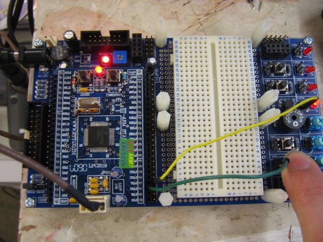
So I finally got onto the next stage of my embedded functional programming project. After scouring the web, the best price/performance ratio I could find for a microcontroller was given by the ET-ARM Stamp made by a company in Thailand. $24.90. Pretty impressive considering the actual microcontroller is a Philips LPC2119 which is a 32-bit ARM deice with 128K Flash ROM, 16K RAM and dozens of analogue and digital IO ports. It's very self-contained - the microcontroller itself requires nothing more than power, a crystal and a couple of capacitors to be up and running, and that's what the ET-ARM board provides. I also bought a small development board with solderless breadboard, switches, LEDs and so on.

So, my first project was to implement a light switch. Here it is:



You can see my finger pressing the button and the LED switched on.

And here's the code running on the microcontroller:

loop = do IO {
            a <- iopin0;
            if band 1024 a>0 then
                ioset0 2048
            else
                ioclr0 2048;
            loop
        }.

start = do IO {
            pinsel0 0;
            iodir0 2048;
            loop
        } 666.

The programming language is my as yet unnamed lazy pure functional language described here.

The code is compiled into C via an intermediate bytecode representation. It's inefficient. Although each 'word' in the code typically compiles to one or two bytecodes, each bytecode expands to around half a dozen 32 bit instructions. (And that can grow if there's lots of lambda lifting going on.) By switching the compiler to thumb mode I got that down to 16 bits per intruction so it's still about a dozen or more bytes per bytecode. Still, with 128K to burn, who's counting? The complete executable is about 48K in size (that's mostly the library, the code itself ). The stack and heap appear to be well behaved. I've managed to run simple logic programs using the list monad without filling the 16K of RAM.

So a quick bit of explanation of the code: the 'main' function is called 'start'. pinsel0 is the C primitive function that sets a bunch of microcontroller pins to function as general I/O ports. iodir0 uses the supplied bitmask to set a bunch of ports to be output ports. (Port 11 in this case.) iopin0 is the function to return the inputs from the I/O ports and ioset0 and ioclr0 set or clear the appropriate I/O ports. Port 10 is connected to the switch and port 11 to the LED. 'band' is my binary 'and' function.

Unlike Haskell, my language is untyped so the 'do' function (it is a function) takes an argument, in this case IO, to specify which monad we're in. I'm using the IO monad to sequence the events (ie. I want the input to be read before the LED state is updates).

And the last thing that needs explaining is the '666'. My IO monad is basically a state monad that makes use of a sequence function 'seq' to ensure that things are evaluated in the right order. 666 is the state that's passed through the monad. It's a dummy value (any value would do) but it's presence is vital as a kind of token that represents the value of the world. For example, if you were to unpack the machinery behind the monad (when I release the code) you'd see that ioclr0 implicitly tries to evaluate the token implicitly returned by iopin0 before executing, ensuring that the switch state is read before the LED state is updated.

Note there's no 'real time' support in the sense that the garbage collector is nothing fancy so it can cause stalls. I make no claim that this is a sensible way to program a microcontroller. :-)

I should mention that I used the free evaluation version of the Keil development system under Windows. It was the slickest microcontroller development environment I've used. (Though my experience of these things isn't great...)

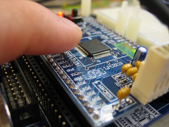
And here's a close up of the microcontroller itself:

Hard to believe that tiny little black square is busy reducing lambda expressions and garbage collecting!

I think my next project will be to design a language better suited to this kind of hardware. I'm thinking of a stream based language like Supercollider. Strongly typed but with guarantees on memory usage deducible at compile time so no garbage collection. I may also make it functional with a degree of support for closures (but in a way that still limits memory usage) and maybe I'll throw S4 into the type system to support a degree of staged computation, very useful when you really need to lighten the load on the target CPU.

Solar Astronomy

I mentioned recently that I'd been volunteering at the local observatory/science museum. You might think there wasn't much astronomy to be done during the day. It turns out you can view Venus. But during the day, if you're armed with the right filters you can also observe one of the most amazing and dynamic astronomical phenomena that are visible: the Sun.

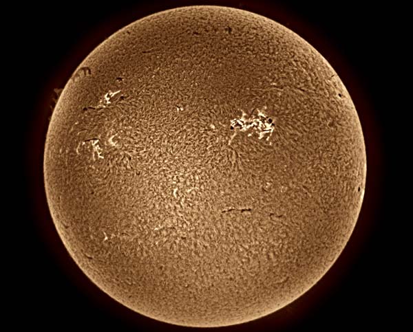
Normally the sun looks like a bright disc of uniform colour. But view it through a hydrogen-α filter and it suddenly transforms into a bizarre alien object. And amazingly you don't need a billion dollar satellite to view the sun this way. A $500 telescope is good enough. Follow that link and you'll see pictures actually taken with that telescope (and subsequently image processed...). You can clearly see solar granulation, filaments, prominences and some of the structure around sunspots.

The problem with solar viewing is that the Sun pumps out vast quantities of energy fairly indiscriminately following a Planck distribution. This tends to overwhelm phenomena that emit at a specific wavelength. So you need an incredibly narrow band pass filter that only allows light at a given wavelength to be transmitted. In this case we were using a filter whose bandwidth was less than 0.1 nanometre to view emissions at 656.3nm caused by electrons dropping from the third to the second energy level in hydrogen atoms.

Making filters this good is itself is an amazing feat. What material could possibly have the correct properties to allow that degree of selectivity? As far as I can make out from the sales blurb, the filter on this telescope is in fact a Fabry-Pérot etalon. Essentially it's two highly reflective (but still slightly transmissive) parallel layers. Consider light travelling perpendicularly through such layers. It might travel straight through. Or it might bounce 2n times before continuing on its way. So the light we see is the sum of light that has bounced 0, 2, 4, 6, ... times. If all of these reflected rays are in phase they'll constructively interfere. Otherwise the infinite sum will be over widely varying phases resulting in destructive interference. So by choosing the correct spacing between the layers we can ensure that only one wavelength (and higher harmonics of it) will be transmitted. You can imagine the difficulty in getting the precise layer separation and that's why these filters can cost many thousands of dollars. And fabrication isn't the only problem - it also needs to be stable even though it has solar energy falling directly onto it.

Anyway, I'm so taken with this solar astronomy stuff I'm going to read this book. And I'll leave you with this link to some even more amazing pictures of the Sun.

(BTW In lieu of having a way to attach my camera to the solar telescope I borrowed the picture from here. Note that the comment is now out of date, the solar neutrino problem has since been solved.)

Defining the Reals

There are a number of schemes for constructing the real numbers starting from set theory. The most common approaches involve constructing the rationals from the ordinal integers and then either forming Dedekind cuts or Cauchy sequences of rationals. But I recently came across an interesting (and fairly new) scheme that I had never seen before. And instead of going via the rationals it jumps straight from the integers to the reals in a simple and intuitive way.



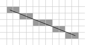
Suppose you have been given the task of plotting a line with gradient m on a computer screen with square pixels. You are told that for each x position on the screen you need to illuminate exactly one pixel in that column. The picture above should illustrate the sort of thing I mean. You need to define a function f such that for each x you illuminate the pixel (x,f(x)). The problem is that different people will choose f differently. Some people might make f(x)=⌊mx⌋. Others might choose f(x)=⌈mx⌉. Some might round mx to the nearest integer giving various choices for what to do when mx is half an odd integer. As the task has only been specified in terms of a gradient, some people might choose to plot an approximation to y=mx+c for various values of c. All of these people will plot different sets of pixels.



But...there are two things that can be said about all of these schemes:

1. for a given m, two reasonable people's choice of the function f will have a bounded difference and
   
2. if two different people are given different gradients then no matter what reasonable scheme they use there will come point, if you travel far enough along the x axis, the two different choices of f(x) will eventually become arbitrarily far apart.
   

In other words, given real numbers m, these crudely specified and rendered plots are a fine enough tool to distinguish between real numbers, but they're not so fine that they distinguish more than the real numbers.

And this intuition gives a nice way to define the real numbers. The idea is to define an almost homomorphism on the integers. f is an almost homomorphism if f(x+y)-f(x)-f(y) is bounded. Clearly the almost-homomorphisms form a group. Amongst the almost homomorphisms are the functions that are themselves bounded. It's not hard to see that according to the scheme I describe above these correspond to a gradient of zero.

The reals are simply the group of almost homomorphisms modulo the bounded functions. That's it!

For more details and proofs see the paper by Arthan. My line plotting example is a modern rendering (no pun intended) of De Morgan's colonnade and fence example.

I first learnt about this from the Wikipedia and the image above was borrowed from the article on the Bresenham line drawing algorithm.

Exceptional Objects

One of my favourite topics in mathematics is the existence of exceptional objects. There have been many articles written on the web about this subject - particularly by John Baez. But I recently came across this article by John Stillwell, in American Mathematical Monthly, that also gives a historical perspective. The connection with classical geometry - Desargue's theorem and Pappus's hexagonal theorem - was also new to me.

Very briefly: mathematics is full of classification theorems. What frequently happens is that objects of a certain type are classified into a bunch of series with a handful of exceptional objects left over. For example the simple finite groups have all been classified and besides the series (such as the cyclic groups of prime order) there are 26 'sporadic' simple groups such as the Monster. The classification of compact Lie groups gives a similar pattern and even the classification of regular polyhedra is similar. Bizarrely, exceptional objects from different branches of mathematics are often related to each other. In fact, the entire classifications from different branches of mathematics are often closely related. And for some reason Dynkin diagrams and octonions seem to play a special role in many of these classifications. The article suggests that the octonions are the "mother of all exceptional objetcs". Anyway, read the article for more information.

I also found this article by the same author on the history of the 120-cell, one of those exceptional regular polyhedra.

Quantum Mechanics and Probability Theory

I've been spending a bit of time thinking about quantum mechanics as an 'exotic' probability theory. It's actually very easy to view quantum mechanics this way and what interests me more is figuring out exactly how quantum mechanics differs from conventional probability theory.

Quantum mechanics looks just like probability theory with a slight twist. Instead of assigning probabilities to events you assign 'amplitudes' which are complex numbers. Computations with these amplitudes are carried out very similarly to computations with probabilitites. If we use a() to mean 'amplitude' a(A or B)=a(A)+a(B) and a(A and B)=a(A)a(B) under similar conditions to those in which P(A or B)=P(A)+P(B) and P(A and B)=P(A)P(B) in conventional probability theory. But these rules for a() only apply when the events A or B remain 'unobserved'. When we actually make observations we switch to a different rule where we now assign probabilities using the rule P(A)=|a(A)|² and these probabilities can be given your favourite probabilistic interpretation.

One interesting thing we can do is recast conventional probability theory so that it looks more like quantum mechanics. For example, consider coin tossing with two outcomes, H and T. We can use these states as the basis for a 2D vector space and write them as |H> and |T>. The outcome of a fair coin toss can be written as 0.5|H>+0.5|T>. When we come to 'observe' the coin its state vector 'collapses' to |H> or |T>. Suppose we have two such coins. Then the joint state space is the tensor product of the state spaces for individual coins. The rule for combining two independent coins into a joint state is the ordinary tensor product. So combining two fair coins gives the state (0.5|H>+0.5|T>)⊗(0.5|H>+0.5|T>)=0.25|H>|H>+0.25|H>|T>+0.25|T>|H>+0.25|T>|T> which can be interpreted as giving the usual probability assigments for fair coin tossing. If we couple the coins together on some way then the joint state might not be a product of individual coin states, ie. we might no longer have independence and their states would be 'entangled'.

Consider a physical process applied to the tossed coin. For example suppose we have a machine that always turns a head over to reveal a tail but only has a 50% chance of turning over a tail. We can think of this as a linear operator mapping |H>→|T> and |T>→0.5|H>+0.5|T>. In this formalism any physical process must be a linear operator given by a stochastic matrix.

Anyone who has studied a little quantum mechanics will recognise many of the phenomena above: the tensorial nature of joint systems, the linearity, the entanglement, the 'collapse' of the state on observation and so on as being nearly identical to features of quantum mechanics. So contrary to popular opinion I think I believe that whatever is interesting about quantum mechanics has nothing to do with any of these features. You can even shoe-horn a variant of the many worlds 'interpretation' of quantum mechanics into probability theory by insisting on the primacy of the state vector and pointing out that when a coin is observed the observation is described by a linear map defined by |H>→|H>|Observer sees H> and |H>→|T>|Observer sees T>.

But almost everyone agrees that quantum mechanics is weird. So how does it really differ from probability theory?

The biggest one is the feature called 'destructive interference'. In conventional probability theory we can combine two states together to make a new state. For example suppose process A generates state |A> and process B generates state |B>. Then we can choose to run either A or B with 50% probability resulting in a new state |C>=p|A>+(1-p)|B>. Suppose A and B are coin states. Then the probability of getting a head when observing state |C> is bounded between the probabilities of getting a head in states A and B. This is a kind of convexity condition. If processes A and B are both roughly fair there's no way of choosing p to 'refine' these states to make another one that's more unfair. And here's the big difference from quantum mechanics. In QM we can choose p to be negative (or any other complex number) and escape from this convexity condition. If we have a quantum coin toss, say |A>=0.6|H>+0.8|T> and |B>=0.8|H>+0.6|T> (in QM the sums of the squares of the moduli are one, not the sums themselves, that's why I chose 0.6 and 0.8), then we can combine them into |C>=-12/7|A>+16/7|B> and get a pure |H> state. We have made the |T> terms cancel out. This is an example of destructive interference. (How do we actually carry out this linear map for arbitrary complex numbers? It's actually very easy - see below.)

One very curious consequence of the above is that we can't ignore low amplitude outcomes. Classicaly, suppose |A>=sqrt(1-e)|H>+e|T> and |B>=sqrt(1-f)|H>+f|T>. If e and f are small enough then no matter what linear combination of |A> and |B> we use to make |C> we can choose to ignore the possibility that we have a head. But in QM, suppose |A>=sqrt(1-|e|²)|H>+e|T> and |B>=sqrt(1-|f|²)|H>+f|T>. Then be carefully crafting |C> from |A> and |B> we can make the probability of getting heads as high as we like.

It's destructive interference that underlies many of the interesting phenomena of QM. For example Shor's factorisation algorithm exploits destructive interference to remove those parts of the quantum computer state that give the wrong answer leaving us with an output that represents a factor.

Non-convexity also leads to other significant consequences. In conventional probability the basis elements |H> and |T> are 'special'. They lie at the extreme 'corners' of the space of possible states and can't be written as stochastic combinations of any other states. But for a quantum coin toss we've shown above that there is no special basis. The state |H> can be written as a linear combination of |A> and |B> just as easily as |A> can be written in terms of |H> and |T> and this is reflected in the fact that we can make a machine that combines |A> and |B> states to make an |H> state. In fact, this is straightforward to observe in the lab. Instead of considering |H> and |T> consider |+> and |-> which correspond to spin up or down states for an electron. Amazingly, if you rotate this state through 90 degrees to make a "spin left" state might get something like (|+>-i|->)/√2. (That answers the question I asked above, just rotate the system.) There is no conventional analogue of this. It is this that is the central problem with Schrödinger's cat. Many people think the problem is that the cat's state becomes something like (|alive>+|dead>)/√2 and can't figure out how to assign meaning to this. But this isn't an issue for QM at all, you can formalise conventional probability so that the cat is described by such a vector and nobody has any difficulty with that. The issue with the Cat is that when the cat is observed it appears to 'collapse' into either the state |dead> or |alive>. Why these two basis elements? In conventional probability these vectors are special. But in QM they are no more special than other vectors.

So in summary - I think that entanglement, wave function collapse and a whole host of other phenomena that are presented as specifically quantum phenomena are nothing but irrelevant distractions and aren't specific to QM at all. The interest value in QM comes from non-convexity and the important problem to solve is the preferred basis problem. (There's also the possibly unanswerable philosophical question of why in Heaven's name the universe looks like a stochastic system with complex numbers for probabilities? And if you're a Bayesian, in what way can a complex number possibly be interpreted as a degree of uncertainty?)

Two Kinds of Mathematics

A recent comment by augustss made me realise that I mentally classify mathematics into two different kinds. I wonder if other mathematicians do the same - so here's your chance to post a comment saying whether or not you agree.

It seems to me that mathematical theorems are either structural theorems or content. By structural I mean that they set up some machinery and show that the machinery does what we expected it to do, and content refers to 'surprising' facts about the mathematical universe. (I think 'structural' is a good choice of word here. 'Content' doesn't feel quite right but the best I could come up with.)

For example, think about a subject like algebraic topology. We start by learning about point set topology. We might define the product topology and then from that show that the projections from the product space to the original space are continuous. These are structural results. They simply tell us that we've defined the product topology in the right way, and the reason why they are the right way is that someone wanted to do topology on the cartesian product of sets and thought hard until they found a way to make this work. They (probably) didn't make a discovery like - hey, there's this amazing topology on the cartesian product that gives continuous projections. They set out to make the product topology in order to prove other stuff, like the way a silversmith or a computer scientist might make tools for themselves for a particular application.

On the other hand, people later started discovering bizarre properties of homotopy groups of spheres. Consider the Hopf fibration which is a beautiful way of building the 3-sphere out of 1-spheres. This was a genuine discovery. It's not just a trivial consequence of the topological machinery but a new result that wasn't plugged in from the beginning. That's what I mean by content.

You invent mathematical machinery, prove structural theorems about it which shows that it does what you want, and then you start discovering interesting results with the machinery. Most branches of mathematics have a mixture of both types of result. In group theory you might prove structural results like the isomorphism theorems which really just show that quotients are what you think they should be. And then you start discovering content like the fact that A_n is simple for n≥5.

Structural theorems tend to be more universal and feel more 'invented'. Content theorems are more specific and feel more 'discovered'. And I'm really talking about a spectrum rather than a binary classification.

Most branches of mathematics have a mixture of the two types of theorem. Typically the structure theorems are used as a tool to discover content. In some sense the content is the end and the structure is the means. But category theory seems different in this regard - it seems to be mainly about structure. Every time I read category theory I see ever more ingenious and abstract tools but I don't really see what I think of as content. What's hard in category theory is getting your head around the definitions and often the theorems are trivial consequences of these. For example consider the Yoneda lemma as described here. This is a pretty challenging result for beginning category theorists. And yet these notes say: "once you have thoroughly understood the statement, you should find the proof straightforward". This exactly fits with what I'm getting at: the theorem is an immediate consequence of the definitions and the proof essentially shows that the machinery does what you'd expect it to do.

Computer science (at least the more formal parts) is a lot like structural mathemtics. It's about inventing machinery (lambdas, coalgebras, state machines) and then proving that machinery does what you expect (diamond property of reductions in lambda calculus etc.). If we compare with group theory the differences become apparent. A mathematician might consider groups in general (general machinery), specialisations of groups such as rings and fields (more machinery) and then specific groups like the Monster or the alternating groups (content). A computer scientist will look at things like untyped lambda calculus, untyped lambda calculus, lambda calculus with this or that extension, but they tend not to look at specific instances in the way that there are specific groups.

Very rarely there is a content theorem that follows from the structural theorems about the tools of computer science. Here's one. 7 binary trees are isomorphic to one. This is a really neat bit of content. This isn't a direct consequence of the definition of trees. When trees were invented nobody thought "what structure can I invent that captures the notion that 7 of them is isomorphic to just one?". This is a discovery, a new result that wasn't plugged in from the beginning.

I guess there is another way to view category theory. As it is the mathematics of structure then in a sense the structure of other branches of mathematics is the content of category theory. It's probably fair to say that one person's content may be another person's content. But it's not unusual for a lecturer to say of their course "the first few weeks will be spent setting up the definitions and machinery and then we'll get onto the real content..."

And now I can reply to augustss. "Real mathematics" is mathematics where from time to time you prove content. And the reason why I said "it's time to get back to some real mathematics" is that much as I've been enjoying computer science lately, I need to see some non-structural content from time to time.

Monads Without Types

People who have just implemented interpreters and compilers are like people who've just had babies - they become monomaniacs incapable of talking about anything else, and showing you their latest pictures at any available opportunity. But I'm going to spare you the pictures. (Hmmm...does blogger.com support the classification of posts by type?)

My typeless pure functional lazy call-by-name language seems to be working out quite well so I thought I'd talk about two aspects of it:

Firstly: my goal has been to construct something as simple as possible that is as powerful as possible. I've basically got it down to just five instructions: push an integer onto the stack, push a pointer to a function, push a duplicate of the nth item down on the stack, push a closure and tidy up a stack frame. Those 5 instructions are then translated into C. Everything else is provided by libraries (eg. plus, minus, seq) or is part of the runtime (ie. garbage collector and the loop that decides which reduction to perform next). The core compiler is basically ten lines of code - the other 300 lines are mainly the parser that has to deal with the quirkiness of any Haskell-like syntax. Yet with this tiny compiler that compiles to just these five operations I've found it possible to write things like a monadic parser, implement monad transformers, and do simple logic programming using the list monad. I'm astonished by how far you can get with so little programming. The moral is, starting from next to nothing you get a lot more bang for your buck with functional programming. (Sometimes it even competes tolerably, performancewise, with Hugs).

Secondly: I thought I'd mention my handling of monads. The compiler only supports three types - integers, pairs and functions so we have no type inferencing tricks to generate the glue to make monads as easy to use as they are in Haskell. Nonetheless I eventually figured out a way to make monads almost as painless as in Haskell. There were two things I needed to do:

(A) Redefine the semantics of " {" and "}". In Haskell anything between "do {" and "}" is glued together using the bind function where bind is overloaded. What I did was similar. Anything between "{" and "}" is glued together using a function. But I don't use the bind function. Instead I define "{ <statements> }" to be a function that uses its argument to bind the statements together. It's then easy to define something like:

do f = f bind.

and we end up with code that looks like Haskell's again. Unfortunately this definition is only useful in the presence of polymorphism because it commits us to using the global 'bind' function. So the way to deal with this is to

(B) Reify monads. I simply define a monad to be the pair (bind:return) where bind and return are the bind and return funtions for the monad. (I use ':' to define pairs as in my language non-null lists are simply pairs constructed form the head and tail of the list.) I can then define do as

do monad f = f (head monad).
return monad = tail monad.

So now the price I have to pay for the lack of types is just that I have to parameterise uses of do and return with the monad. This isn't too onerous, for example you get code looking like:

putLine l = if l then
                    doIO {
                        putChar (head l);
                        putLine (tail l)
                    }
                else
                    returnIO 0.

where I've defined doIO = do IO etc.

It gets a little more complex with monad transformers. As monads are reified, a monad transformer in my language is an actual function that maps a monad to a monad. For example, here's part of the definition of the StateT monad transformer:

returnStateT monad x s = return monad (x:s).
bindStateT monad m k s = bind monad (m s) (\as -> k (head as) (tail as)).
doStateT monad f = f (bindStateT monad).
-- Actually construct the transformed monad.
StateT monad = bindStateT monad : returnStateT monad.

In some ways these definitions are actually simpler than the corresponding Haskell definitions. In Haskell you communicate information to the compiler about which bind and return to use by your choice of type. So you find yourself repeatedly wrapping and unwrapping objects (eg. using runStateT). No such issue here, a sequence of statements in the state monad can simply be applied immediately to the input state.

Anyway, the monad transformer examples I came up with earlier now carry over to my new language like so:

prog = do (StateT State) {
            liftStateT State (modify (plus 1));
            a <- liftStateT State get;
            modifyT State (plus 10);
            b <- getT State;
            liftStateT State $ put (a+b);
            c <- getT State;
            return (StateT State) $ c+1
       }.

Note that I chose to make everything explicit. I could easily have made local definitions like lift = liftStateT State to make things look more like Haskell.

Anyway, I'm pretty pleased. With a few hours of coding here and there over a period of two weeks I've written my first compiler of standalone executables in 20 years and it's already at the stage where it wouldn't be hard to port its own compiler to itself. (My previous compiler was an adventure game DSL written in BASIC and based on the one here (though I don't think the acronym 'DSL' existed then). I also implemented Forth on a Psion II a bit later but it's debatable whether you'd call indirect threading by the name 'compilation'.)

I'll probably put a release on my web site some time in the next week. Not that it's actually useful for anything...

And all this computer science is too much. I really must get back to some real mathematics some time soon...

Writing a pure functional lazy call-by-name compiler

There are lots of minimal functional language/lambda expression evaluators out there, so instead I thought I'd write one that actually compiled to standalone C. But by accident it seems to have grown and I now have a 'typeless' Haskell, or at least a language with ML type grammar, lazy evaluation and call-by-name, primitive monad support and only two types - integers and lists. I'm now at the stage where I can compile pieces of code like this:

return a s = a : s.
bind x f s = let vs = x s in seq vs ((f (head vs) (tail vs))).
bind' x f s = bind x (\a b -> f b) s.

contains x = if x
               (if (head x==81) 1 (contains (tail x)))
               0.

getLine = do {
           c <- getChar;
           if (c==10)
                 (return 0)
                 do {
                   l <- getLine;
                   return (c : l)
                 }

          }.

putLine l = if l
               do {
                   putChar (head l);
                   putLine (tail l)
               }
               (return 0).

prog = do {
           a <- getLine;
           if (contains a) ( do { putLine a; putChar 10 }) (return 0);
           prog
       }.

start = prog 666.

This piece of code does the same as "grep Q" and amazingly doesn't leak memory and could probably outrun a snail (just). When I tidy it up and fix the bugs I'll release the compiler on my web page.

It's been one hell of a learning experience. The main thing I've learnt is that those compiler writers are damn clever people. But I also learnt other things like: even the most innocent looking expressions can gobble up vast amounts of memory in a lazy language, it's really heard to debug lazy programs even when you have complete freedom to make your compiler emit whatever 'instrumentation' you want, garbage collection is more subtle than I thought and Haskell has a weird grammar. On the other hand, some things were easier than I expected. Dealing with lambda expressions looks hard at first - but lambda lifting is very easy to implement so that once you have a way of compiling equations, lambdas come for free. And ultimately it's incredible how much stuff you can get for nothing. The core compiler is miniscule - it knows how to compile one operation - function application. The rest is syntactic sugar or part of the library that the C code links to.

My ultimate goal is to get my compiler to emit self-contained C programs that are as small as possible. I'd like to take these programs and make them run on a microcontroller like the one in this robot I built last year. It has 1K of RAM, 8K of program space and runs at 8MHz, which may be enough for a simple light following algorithm. (In assembler it'd be about 100 bytes long and use 2 or 3 bytes of RAM.) I don't want to actually achieve anything useful - I'm too much of a mathematician to want to do that. I just want to construct an example of what I see as an extreme form of computational perversity: a pure language with no side effects having actual side effects in the physical world.